6 Multigroup Analysis
6.1 Introduction to Multigroup Analysis
Often in ecology we wish to compare the results from two or more groups. These groups could reflect experimental treatments, different sites, different sexes, or any number of types of organization. The ultimate goal of such an analysis is to ask whether the relationships among predictor and response variables vary by group.
Historically, such a goal would be captured through the application of a statistical interaction. For example, does the effect of pesticide on invertebrate biomass change as function of where the pesticide is applied? This model might look something like this:
\[biomass = pesticide \times location\]
A significant interaction between \(pesticide \times location\) would indicate that the effect of pesticide application on invertebrate biomass indeed varies by location. It would of course then be up to the author to use their knowledge of the system to speculate why this is.
In the event that the interaction is not statistically significant, the author would conclude that the effect of pesticide is invariant to location. The author could instead generalize the effects of pesticide, such that it’s expected to have the same magnitude of effect regardless of where it’s applied.
A multigroup model is essentially the same principle, but instead of focusing on a single response, the interaction is applied across the entire structural equation model. In other words, it asks if not just one but all coefficients are the same or different across groups. In a sense, it can be thought of as a “model-wide” interaction, and, in fact, this is how we will treat it later using a piecewise approach.
Of course, you might ask: why not simply fit the same model structure to different subsets of the data? Unfortunately, this would not allow you to identify which paths change based on the group and which do not, which could be key insight. Rather, one would have to compare the magnitude and standard errors of each pair of coefficients manually, rather than through a formal statistical procedure.
The application of multigroup models differs between a global estimation (i.e., variance-covariance based SEM) and local estimation (i.e., piecewise SEM), but they adhere to the same idea of identifying which paths have the same effect across groups and which paths vary depending on the group.
In this chapter, we will work through both approaches and then compare/contrast the output.
6.2 Multigroup Analysis using Global Estimation
Multigroup modeling using global estimation begins with the estimation of two models: one in which all parameters are allowed to differ between groups, and one in which all parameters are fixed to those obtained from analysis of the pooled data across groups. We call the first model the “free” model since all parameters are free to vary and the second the “constrained” model since each path, regardless of its group, is constrained to a single value determined by the entire dataset.
If the two models are not significantly different, and the latter fits the data well, then one can assume there is no variation in the path coefficients by group and multigroup approach is not necessary. In this case, the output from the constrained model would be reported.
If they are, then the exercise shifts towards understanding which paths are the same and which are different. This is achieved by sequentially constraining the coefficients of each path and re-fitting the model.
Let’s illustrate this procedure using a random example using three variables–\(x\), \(y\), and \(z\)–in two groups: “a” and “b.”
set.seed(111)

dat <- data.frame(x = runif(100), group = rep(letters[1:2], each = 50))

dat$y <- dat$x + runif(100)

dat$z <- dat$y + runif(100)
In this example, we suppose a simple mediation model: \(x -> y -> z\), and that all three variables are correlated to some degree so that this model makes sense.
We can use lavaan to fit the “free” model. The key is allowing the coefficients to vary by specifying the group = argument:
multigroup.model <- '
y ~ x
z ~ y
'

library(lavaan)

multigroup1 <- sem(multigroup.model, dat, group = "group")
We can then obtain the summary of the multigroup analysis:
summary(multigroup1)## lavaan 0.6-9 ended normally after 38 iterations
##
## Estimator ML
## Optimization method NLMINB
## Number of model parameters 12
##
## Number of observations per group:
## a 50
## b 50
##
## Model Test User Model:
##
## Test statistic 0.092
## Degrees of freedom 2
## P-value (Chi-square) 0.955
## Test statistic for each group:
## a 0.049
## b 0.043
##
## Parameter Estimates:
##
## Standard errors Standard
## Information Expected
## Information saturated (h1) model Structured
##
##
## Group 1 [a]:
##
## Regressions:
## Estimate Std.Err z-value P(>|z|)
## y ~
## x 0.771 0.163 4.734 0.000
## z ~
## y 1.080 0.126 8.577 0.000
##
## Intercepts:
## Estimate Std.Err z-value P(>|z|)
## .y 0.684 0.088 7.745 0.000
## .z 0.463 0.140 3.313 0.001
##
## Variances:
## Estimate Std.Err z-value P(>|z|)
## .y 0.080 0.016 5.000 0.000
## .z 0.092 0.018 5.000 0.000
##
##
## Group 2 [b]:
##
## Regressions:
## Estimate Std.Err z-value P(>|z|)
## y ~
## x 1.240 0.135 9.182 0.000
## z ~
## y 0.897 0.086 10.465 0.000
##
## Intercepts:
## Estimate Std.Err z-value P(>|z|)
## .y 0.349 0.078 4.460 0.000
## .z 0.612 0.092 6.654 0.000
##
## Variances:
## Estimate Std.Err z-value P(>|z|)
## .y 0.082 0.016 5.000 0.000
## .z 0.081 0.016 5.000 0.000Note that, unlike the typical lavaan output, the printout is now organized by group, with separate coefficients for each path in each group. Because this model is allowed to vary, the coefficient for the \(x -> y\) path in group “a” is different, for example, from that reported for group “b”.
Next, we fit the constrained model by specifying the additional argument group.equal = c("intercepts", "regressions"). This argument fixes both the intercepts and path coefficients in each group to be the same.
multigroup1.constrained <- sem(multigroup.model, dat, group = "group", group.equal = c("intercepts", "regressions"))

summary(multigroup1.constrained)
## lavaan 0.6-9 ended normally after 29 iterations
##
## Estimator ML
## Optimization method NLMINB
## Number of model parameters 12
## Number of equality constraints 4
##
## Number of observations per group:
## a 50
## b 50
##
## Model Test User Model:
##
## Test statistic 9.951
## Degrees of freedom 6
## P-value (Chi-square) 0.127
## Test statistic for each group:
## a 5.541
## b 4.410
##
## Parameter Estimates:
##
## Standard errors Standard
## Information Expected
## Information saturated (h1) model Structured
##
##
## Group 1 [a]:
##
## Regressions:
## Estimate Std.Err z-value P(>|z|)
## y ~
## x (.p1.) 1.046 0.108 9.678 0.000
## z ~
## y (.p2.) 0.960 0.072 13.413 0.000
##
## Intercepts:
## Estimate Std.Err z-value P(>|z|)
## .y (.p6.) 0.499 0.061 8.219 0.000
## .z (.p7.) 0.570 0.078 7.283 0.000
##
## Variances:
## Estimate Std.Err z-value P(>|z|)
## .y 0.087 0.017 5.000 0.000
## .z 0.094 0.019 5.000 0.000
##
##
## Group 2 [b]:
##
## Regressions:
## Estimate Std.Err z-value P(>|z|)
## y ~
## x (.p1.) 1.046 0.108 9.678 0.000
## z ~
## y (.p2.) 0.960 0.072 13.413 0.000
##
## Intercepts:
## Estimate Std.Err z-value P(>|z|)
## .y (.p6.) 0.499 0.061 8.219 0.000
## .z (.p7.) 0.570 0.078 7.283 0.000
##
## Variances:
## Estimate Std.Err z-value P(>|z|)
## .y 0.089 0.018 5.000 0.000
## .z 0.083 0.017 5.000 0.000This output is slightly different from the first: the coefficients are reported by group, but they are now identical between groups (e.g., \(\gamma_x\) in group “a” = \(\gamma_x\) in group “b”). The constrained paths are indicated by a parenthetical next to the path (e.g., (.p1.) for path 1).
Both the constrained and free models fit the data well based on the \(\chi^2\) statistic, and we can formally compare the two using a Chi-squared difference test:
anova(multigroup1, multigroup1.constrained)## Chi-Squared Difference Test
##
## Df AIC BIC Chisq Chisq diff Df diff Pr(>Chisq)
## multigroup1 2 95.392 126.65 0.0921
## multigroup1.constrained 6 97.251 118.09 9.9508 9.8588 4 0.04288 *
## ---
## Signif. codes: 0 '***' 0.001 '**' 0.01 '*' 0.05 '.' 0.1 ' ' 1The significant P-value implies that the free and constrained models are significantly different. In other words, some paths vary while others may not. If the models were not significantly different, then one would conclude that the constrained model is equivalent to the free model, or that the coefficients would not vary by group, and it would be fair to analyze the pooled data in a single global model.
However, this is the not the case for this example, and we can now undergo the process of introducing and releasing constraints to try and identify which path varies between groups. In this simplified example, we have two choices: \(x -> y\), and \(y -> z\). Let’s focus on \(x -> y\) first.
We can introduce a single constraint by modifying the model formula and re-fitting the model:
multigroup.model2 <- '
y ~ c("b1", "b1") * x
z ~ y
'

multigroup2 <- sem(multigroup.model2, dat, group = "group")
The string c("b1", "b1") gives the path the name b1 and ensures the coefficient is equal between the two groups (hence the two entries).
If we use a Chi-squared difference test as before:
anova(multigroup1, multigroup2)## Chi-Squared Difference Test
##
## Df AIC BIC Chisq Chisq diff Df diff Pr(>Chisq)
## multigroup1 2 95.392 126.65 0.0921
## multigroup2 3 98.188 126.84 4.8881 4.796 1 0.02853 *
## ---
## Signif. codes: 0 '***' 0.001 '**' 0.01 '*' 0.05 '.' 0.1 ' ' 1We find that the models are still significantly different, implying that the path between \(x -> y\) should not be constrained and instead that it should be left to vary among groups.
We can repeat this exercise with the second path, \(y -> z\):
multigroup.model3 <- '
y ~ x
z ~ c("b2", "b2") * y
'

multigroup3 <- sem(multigroup.model3, dat, group = "group")

anova(multigroup1, multigroup3)
## Chi-Squared Difference Test
##
## Df AIC BIC Chisq Chisq diff Df diff Pr(>Chisq)
## multigroup1 2 95.392 126.65 0.0921
## multigroup3 3 94.823 123.48 1.5230 1.4309 1 0.2316In this case, there is not a significant difference between the two models (P = 0.23), implying that the is no difference in the fit of the constrained model and the unconstrained model and that this constraint is valid.
If we were to select across these three alternatives, we would select the third model in which \(x -> y\) is allowed to vary and \(y -> z\) is constrained among groups. It’s key to note that this model also fits the data well based on the \(\chi^2\) statistic; if not, then like all poor-fitting path models (multigroup or otherwise) it would be unwise to present and draw conclusions from it.
This exercise of relaxing and imposing constraints is potentially very exploratory and could become exhaustive with more complicated models (i.e., one with lots of paths to potentially constrain/relax). Users should refrain from constraining and relaxing all paths and then choosing the most parsimonious model. Instead, choosing which paths to constrain should be motivated by the question: for example, we might expect some effects to be universal (e.g., temperature on metabolic rate) but not others (e.g., the effect of pesticide may vary depending on the history of application at various sites).
Critically, the degrees of freedom for the model do not change based on the number of groups because coefficients are estimated from variance-covariance matrices with the same dimensions. However, sample size must be sufficiently large to estimate all the parameters within each group with minimal bias. While this is true for all structural equation models, it is especially true where parameters are estimated from covariances derived from different subsets (groups) that do not have the same replication.
Standardized coefficients also present a challenge. Because variances are likely to be unequal among groups (unless they are drawn from the same population), the standardized coefficient must be computed on a per group basis, even if the unstandardized coefficient is constrained to the global value. Both packages for SEM will do this automatically, so you may notice that the standardized solutions may–and more than often will–vary even among constrained paths.
6.3 Multigroup Analysis Using Local Estimation
The goal of multigroup analysis using local estimation is identical to that of global estimation: to identify whether a single global model is sufficient to describe the data, or whether some or all paths vary by some grouping variable. The difference lies in execution: while lavaan is a back-and-forth manual process of relaxing and constraining paths, piecewiseSEM tests constraints and automatically selects the best output for your data.
The upside is that the arduous and somewhat cumbersome process of specifying constraints is taken care of; the downside is that manually constraining particular paths is not possible at this time, although forthcoming work by Shipley and Douma will make this possible.
The first step in the local estimation process is to implement a model-wide interaction. In other words, every term in the model interacts with the grouping variable. If the interaction is significant, then the path is free to vary by group; if not, then the path takes on the estimate from the global dataset. In this way, the piecewise multigroup procedure breaks down into a series of classic interaction terms: it is literally and figuratively the model-wide interaction we discussed at the beginning of this chapter
Consider our previous example fitted using lavaan. In a piecewise approach, we would first model the interaction between \(x \times group\) to see whether the effect of \(x\) on \(y\) should vary by group:
anova(lm(y ~ x * group, dat))## Analysis of Variance Table
##
## Response: y
## Df Sum Sq Mean Sq F value Pr(>F)
## x 1 8.2740 8.2740 97.9518 2.475e-16 ***
## group 1 0.2772 0.2772 3.2811 0.07321 .
## x:group 1 0.3974 0.3974 4.7051 0.03254 *
## Residuals 96 8.1091 0.0845
## ---
## Signif. codes: 0 '***' 0.001 '**' 0.01 '*' 0.05 '.' 0.1 ' ' 1In this case, the effect of \(x\) on \(y\) depends on \(group\) (a significant interaction term). We would then estimate the effect of \(x\) and \(y\) for each subset of the data, and report the coefficients separately. =
Next, we evaluate the effect of \(y\) on \(z\) by group:
anova(lm(z ~ y * group, dat))## Analysis of Variance Table
##
## Response: z
## Df Sum Sq Mean Sq F value Pr(>F)
## y 1 15.8899 15.8899 176.3764 <2e-16 ***
## group 1 0.0366 0.0366 0.4066 0.5252
## y:group 1 0.1271 0.1271 1.4107 0.2379
## Residuals 96 8.6487 0.0901
## ---
## Signif. codes: 0 '***' 0.001 '**' 0.01 '*' 0.05 '.' 0.1 ' ' 1The second interaction between \(y \times group\) in predicting \(z\) is non-significant, indicating that the effect of \(y\) on \(z\) does not depend on \(group\). We would then estimate the effect of \(y\) on \(z\) using the entire dataset and report that single constrained coefficient across all groups.
The implementation of this approach in piecewiseSEM is very straightforward: first, build the model using psem, then use the function multigroup to perform the multigroup analysis.
library(piecewiseSEM)

pmodel <- psem(
  lm(y ~ x, dat),
  lm(z ~ y, dat)
)
The multigroup function has an argument group = which, as in lavaan, accepts the column name of the grouping factor:
(pmultigroup <- multigroup(pmodel, group = "group"))##
## Structural Equation Model of pmodel
##
## Groups = group [ a, b ]
##
## ---
##
## Global goodness-of-fit:
##
## Fisher's C = 0.301 with P-value = 0.86 and on 2 degrees of freedom
##
## ---
##
## Model-wide Interactions:
##
## Response Predictor Test.Stat DF P.Value
## y x:group 8.3 1 0.0325 *
## z y:group 15.5 1 0.2379
##
## y -> z constrained to the global model
##
## ---
##
## Group [a] coefficients:
##
## Response Predictor Estimate Std.Error DF Crit.Value P.Value Std.Estimate
## y x 0.7712 0.1662 48 4.6387 0 0.5563 ***
## z y 0.9652 0.0726 98 13.2931 0 0.6895 *** c
##
## Group [b] coefficients:
##
## Response Predictor Estimate Std.Error DF Crit.Value P.Value Std.Estimate
## y x 1.2404 0.1379 48 8.9963 0 0.7923 ***
## z y 0.9652 0.0726 98 13.2931 0 0.8914 *** c
##
## Signif. codes: 0 '***' 0.001 '**' 0.01 '*' 0.05 c = constrainedIf we examine the output, we see the output table of model-wide interactions. It’s important to note that the package uses car::Anova with type = "II" sums-of-squares to estimate the interactions by default, but other types (e.g., type III) are accepted using the test.type = argument (or type I using the base anova function).
As above, only the path from \(x\) -> \(y\) is significantly different among groups. In this case, the function explicitly reports that the path y -> z constrained to the global model.
Next, as in lavaan, are the coefficient tables for each group. Values that have been constrained are the same between the two models and indicated with a c at the end of the row, while the unconstrained path from \(x -> y\) is different between groups “a” and “b”.
It’s important to note that the standardized coefficients do differ for each group even though the paths are constrained. Again, this is because the variance differs between groups. Thus the standardization:
$$\beta_{std} = \beta*\left( \frac{sd_{x}}{sd_{y}} \right)$$must consider only the standard deviation of x and y from their respective groups, even though \(\beta\) is derived from the entire dataset.
Finally, near the top is the global goodness-of-fit test based on Fisher’s C. In this case, global constraints have been added as offset to the tests of directed separation.
For comparison’s sake, let’s look at the output from the lavaan multigroup model and the piecewiseSEM one:
standardizedSolution(multigroup3)## lhs op rhs group label est.std se z pvalue ci.lower ci.upper
## 1 y ~ x 1 0.556 0.090 6.197 0.000 0.380 0.732
## 2 z ~ y 1 b2 0.728 0.054 13.556 0.000 0.623 0.833
## 3 y ~~ y 1 0.690 0.100 6.912 0.000 0.495 0.886
## 4 z ~~ z 1 0.470 0.078 6.014 0.000 0.317 0.623
## 5 x ~~ x 1 1.000 0.000 NA NA 1.000 1.000
## 6 y ~1 1 2.012 0.406 4.953 0.000 1.216 2.808
## 7 z ~1 1 1.336 0.259 5.158 0.000 0.828 1.844
## 8 x ~1 1 1.971 0.000 NA NA 1.971 1.971
## 9 y ~ x 2 0.792 0.044 18.167 0.000 0.707 0.878
## 10 z ~ y 2 b2 0.843 0.036 23.508 0.000 0.773 0.913
## 11 y ~~ y 2 0.372 0.069 5.387 0.000 0.237 0.508
## 12 z ~~ z 2 0.289 0.060 4.782 0.000 0.171 0.408
## 13 x ~~ x 2 1.000 0.000 NA NA 1.000 1.000
## 14 y ~1 2 0.742 0.213 3.480 0.001 0.324 1.160
## 15 z ~1 2 1.045 0.210 4.976 0.000 0.633 1.456
## 16 x ~1 2 1.650 0.000 NA NA 1.650 1.650pmultigroup$group.coefs## $a
## Response Predictor Estimate Std.Error DF Crit.Value P.Value Std.Estimate
## 1 y x 0.7712 0.1662 48 4.6387 0 0.5563 ***
## 2 z y 0.9652 0.0726 98 13.2931 0 0.6895 ***
##
## 1
## 2 c
##
## $b
## Response Predictor Estimate Std.Error DF Crit.Value P.Value Std.Estimate
## 1 y x 1.2404 0.1379 48 8.9963 0 0.7923 ***
## 2 z y 0.9652 0.0726 98 13.2931 0 0.8914 ***
##
## 1
## 2 cYou’ll note that the outputs are roughly equivalent (owing to slight differences in the estimation procedures for each package). Critically, the coefficient for the path from \(z -> y\) is the same in both groups.
6.4 Grace & Jutila (1999): A Worked Example
Let’s now turn to a real example from Grace & Jutila (1999). While the original paper fit a far more complicated model than we will, the following simplified model demonstrates the approach well.
In their study, the authors were interested in the controls of on plant species density in Finnish meadows. In this worked example, we will consider only elevation and total biomass in their effects on density, plus an effect of elevation on biomass:
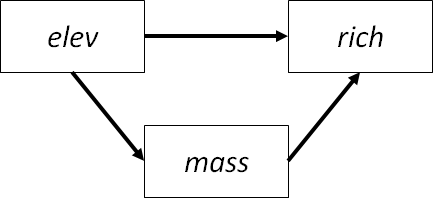
Moreover, they repeated their observations in two treatments: grazed and ungrazed meadows. Grazing will serve as the grouping variable for our multigroup analysis.
The data are included in piecewiseSEM so let’s load it:
data(meadows)First, let’s construct the “free” model in lavaan:
jutila_model <- '
rich ~ elev + mass
mass ~ elev
'

jutila_lavaan_free <- sem(jutila_model, meadows, group = "grazed")

summary(jutila_lavaan_free)
## lavaan 0.6-9 ended normally after 53 iterations
##
## Estimator ML
## Optimization method NLMINB
## Number of model parameters 14
##
## Number of observations per group:
## 1 165
## 0 189
##
## Model Test User Model:
##
## Test statistic 0.000
## Degrees of freedom 0
## Test statistic for each group:
## 1 0.000
## 0 0.000
##
## Parameter Estimates:
##
## Standard errors Standard
## Information Expected
## Information saturated (h1) model Structured
##
##
## Group 1 [1]:
##
## Regressions:
## Estimate Std.Err z-value P(>|z|)
## rich ~
## elev 0.073 0.010 7.232 0.000
## mass -0.001 0.002 -0.424 0.672
## mass ~
## elev -1.203 0.470 -2.559 0.010
##
## Intercepts:
## Estimate Std.Err z-value P(>|z|)
## .rich 7.169 0.708 10.126 0.000
## .mass 260.855 26.764 9.746 0.000
##
## Variances:
## Estimate Std.Err z-value P(>|z|)
## .rich 12.459 1.372 9.083 0.000
## .mass 28057.590 3089.039 9.083 0.000
##
##
## Group 2 [0]:
##
## Regressions:
## Estimate Std.Err z-value P(>|z|)
## rich ~
## elev 0.088 0.011 7.988 0.000
## mass -0.007 0.001 -5.465 0.000
## mass ~
## elev -3.274 0.554 -5.908 0.000
##
## Intercepts:
## Estimate Std.Err z-value P(>|z|)
## .rich 11.349 0.750 15.139 0.000
## .mass 451.732 24.949 18.107 0.000
##
## Variances:
## Estimate Std.Err z-value P(>|z|)
## .rich 14.384 1.480 9.721 0.000
## .mass 43567.994 4481.792 9.721 0.000In this example, the model goodness-of-fit fit can’t be determined because the model is saturated (df = 0). This is key moving forward because constraining paths will free up degrees of freedom with which to obtain a test statistic.
Also note the warning message above variances being a factor 1000 times larger than others. This can be problematic for the estimation of the variance-covariance matrix. The simple solution is the use the function scale or add/subtract a constant to reduce these values before fitting the model.
Let’s begin by constraining all paths:
jutila_lavaan_constrained <- sem(jutila_model, meadows, group = "grazed", group.equal = c("intercepts", "regressions"))

anova(jutila_lavaan_free, jutila_lavaan_constrained)
## Chi-Squared Difference Test
##
## Df AIC BIC Chisq Chisq diff Df diff Pr(>Chisq)
## jutila_lavaan_free 0 6666.2 6720.3 0.000
## jutila_lavaan_constrained 5 6754.4 6789.2 98.261 98.261 5 < 2.2e-16
##
## jutila_lavaan_free
## jutila_lavaan_constrained ***
## ---
## Signif. codes: 0 '***' 0.001 '**' 0.01 '*' 0.05 '.' 0.1 ' ' 1The model is significantly different from the unconstrained model we fit previously (P < 0.001), implying that some paths could be constrained. Note that, by constraining all the coefficients, we now have 5 degrees of freedom to evaluate model fit. (However, if we were to examine it, we would find that it is a poor fit, implying that some path coefficients must vary among groups.)
The next step is to sequentially relax and constrain paths:
jutila_model2 <- '
rich ~ elev + mass
mass ~ c("b1", "b1") * elev
'

jutila_lavaan2 <- sem(jutila_model2, meadows, group = "grazed")

anova(jutila_lavaan_free, jutila_lavaan2)
## Chi-Squared Difference Test
##
## Df AIC BIC Chisq Chisq diff Df diff Pr(>Chisq)
## jutila_lavaan_free 0 6666.2 6720.3 0.0000
## jutila_lavaan2 1 6672.2 6722.5 8.0301 8.0301 1 0.004601 **
## ---
## Signif. codes: 0 '***' 0.001 '**' 0.01 '*' 0.05 '.' 0.1 ' ' 1The model is still a poor fit, and it is significantly different from the “free” model (P = 0.005). In this case, we would conclude that the \(elev -> mass\) path should not be constrained.
Let’s repeat for the next two paths:
# elev -> rich
jutila_model3 <- '
rich ~ c("b2", "b2") * elev + mass
mass ~ elev
'

jutila_lavaan3 <- sem(jutila_model3, meadows, group = "grazed")

anova(jutila_lavaan_free, jutila_lavaan3)
## Chi-Squared Difference Test
##
## Df AIC BIC Chisq Chisq diff Df diff Pr(>Chisq)
## jutila_lavaan_free 0 6666.2 6720.3 0.0000
## jutila_lavaan3 1 6665.1 6715.4 0.9477 0.94767 1 0.3303# mass -> rich
jutila_model4 <- '
rich ~ elev + c("b3", "b3") * mass
mass ~ elev
'
jutila_lavaan4 <- sem(jutila_model4, meadows, group = "grazed")
anova(jutila_lavaan_free, jutila_lavaan4)## Chi-Squared Difference Test
##
## Df AIC BIC Chisq Chisq diff Df diff Pr(>Chisq)
## jutila_lavaan_free 0 6666.2 6720.3 0.0000
## jutila_lavaan4 1 6673.6 6723.9 9.4642 9.4642 1 0.002095 **
## ---
## Signif. codes: 0 '***' 0.001 '**' 0.01 '*' 0.05 '.' 0.1 ' ' 1Of these two paths, it seems the first: \(elev -> rich\), is not significantly different from the “free” model, implying that this path could be constrained. Oppositely, the significant difference between the “free” model and one in which the \(mass -> rich\) path is constrained suggests that constraining this path is not supported.
Let’s check the fit of the model with the one constrait on \(elev -> rich\):
summary(jutila_lavaan3)## lavaan 0.6-9 ended normally after 53 iterations
##
## Estimator ML
## Optimization method NLMINB
## Number of model parameters 14
## Number of equality constraints 1
##
## Number of observations per group:
## 1 165
## 0 189
##
## Model Test User Model:
##
## Test statistic 0.948
## Degrees of freedom 1
## P-value (Chi-square) 0.330
## Test statistic for each group:
## 1 0.435
## 0 0.513
##
## Parameter Estimates:
##
## Standard errors Standard
## Information Expected
## Information saturated (h1) model Structured
##
##
## Group 1 [1]:
##
## Regressions:
## Estimate Std.Err z-value P(>|z|)
## rich ~
## elev (b2) 0.080 0.007 10.717 0.000
## mass -0.000 0.002 -0.297 0.767
## mass ~
## elev -1.203 0.470 -2.559 0.010
##
## Intercepts:
## Estimate Std.Err z-value P(>|z|)
## .rich 6.795 0.596 11.408 0.000
## .mass 260.855 26.764 9.746 0.000
##
## Variances:
## Estimate Std.Err z-value P(>|z|)
## .rich 12.492 1.375 9.083 0.000
## .mass 28057.590 NA
##
##
## Group 2 [0]:
##
## Regressions:
## Estimate Std.Err z-value P(>|z|)
## rich ~
## elev (b2) 0.080 0.007 10.717 0.000
## mass -0.008 0.001 -5.999 0.000
## mass ~
## elev -3.274 0.554 -5.908 0.000
##
## Intercepts:
## Estimate Std.Err z-value P(>|z|)
## .rich 11.754 0.624 18.831 0.000
## .mass 451.732 24.949 18.107 0.000
##
## Variances:
## Estimate Std.Err z-value P(>|z|)
## .rich 14.423 1.484 9.721 0.000
## .mass 43567.993Now the model fits the data well (P = 0.330), and we have, through an iterative procedure of imposing and relaxing constraints, determined which paths differ among groups (\(elev -> mass\), \(mass -> rich\)) and which do not (\(elev -> rich\)).
Now let’s confirm this by fitting the model in piecewiseSEM:
jutila_psem <- psem(
  lm(rich ~ elev + mass, meadows),
  lm(mass ~ elev, meadows)
)

multigroup(jutila_psem, group = "grazed")
##
## Structural Equation Model of jutila_psem
##
## Groups = grazed [ 1, 0 ]
##
## ---
##
## Global goodness-of-fit:
##
## Fisher's C = NA with P-value = NA and on 0 degrees of freedom
##
## ---
##
## Model-wide Interactions:
##
## Response Predictor Test.Stat DF P.Value
## rich elev:grazed 1556.7 1 0.3358
## rich grazed:mass 1556.7 1 0.0026 **
## mass elev:grazed 1416938.0 1 0.0055 **
##
## elev -> rich constrained to the global model
##
## ---
##
## Group [1] coefficients:
##
## Response Predictor Estimate Std.Error DF Crit.Value P.Value Std.Estimate
## rich elev 0.0731 0.0081 351 8.9882 0.0000 0.4967 ***
## rich mass -0.0007 0.0017 162 -0.4198 0.6752 -0.0291
## mass elev -1.2028 0.4728 163 -2.5438 0.0119 -0.1954 *
##
## c
##
##
##
## Group [0] coefficients:
##
## Response Predictor Estimate Std.Error DF Crit.Value P.Value Std.Estimate
## rich elev 0.0731 0.0081 351 8.9882 0 0.3933 ***
## rich mass -0.0072 0.0013 186 -5.4216 0 -0.3222 ***
## mass elev -3.2735 0.5571 187 -5.8764 0 -0.3948 ***
##
## c
##
##
##
## Signif. codes: 0 '***' 0.001 '**' 0.01 '*' 0.05 c = constrainedAs in our analysis in lavaan, the multigroup function has identified the \(elev -> rich\) path as the only one in which coefficients do not differ among groups (again, denoted by a c next to the output). Thus, in the output, that coefficient is the same between groups; otherwise, the coefficients vary depending on whether the meadows is grazed or ungrazed. Moreover, it seems some of the paths differ in their statistical significance: the \(rich -> mass\) is not significant in the grazed meadows, but is significant in the ungrazed meadows. So not only do the coefficients differ, but the model structure as well.
You’ll note that the piecewiseSEM output does not return a goodness-of-fit test because the model is saturated (i.e., no missing paths). While constraints are incorporated in terms of offsets (i.e., fixing model coefficients), unlike global estimation, this procedure does not provide new information with which to test goodness-of-fit. This is a limitation of local estimation that extends beyond multigroup modeling to any piecewise model.
To draw inference about the study system, we would say that two paths differ among groups and one path does not. We would then report the two path models parameterized using the coefficient output (with the \(elev -> rich\) path having the same coefficient in both groups). We would conclude that richness is affected by elevation and biomass under ungrazed conditions, but not under grazed conditions, where only elevation directly influences richness.
6.5 References
Grace, J. B., & Jutila, H. (1999). The relationship between species density and community biomass in grazed and ungrazed coastal meadows. Oikos, 398-408.