2 Global Estimation
2.1 What is (Co)variance?
The building block of the global estimation procedure for SEM is variance, specifically the covariance between variables. Before we delve into the specifics of this procedure, it’s worth reviewing the basics of variance and covariance.
Variance is the degree of spread in a set of data. Formally, it captures the deviation of each point from the mean value across all points. Consider the variable \(x\). The variance of \(x\) is calculated as:
\[VAR_{x} = \frac{\sum(x_{i} - \overline{x})^2}{n-1}\]
where \(x_{i}\) is each sample value, \(\overline{x}\) is the sample mean, and \(n\) is the sample size.
Similarly, for the response \(y\):
\[VAR_{y} = \frac{\sum(y_{i} - \overline{y})^2}{n-1}\]
Note that, regardless of the actual scale of the variables, variances are always positive (due to the squared term). The larger the variance, the more spread out the data are around the mean.
Covariance is a measure of the dependency between two variables. Covariance can be formalized as:
\[COV_{xy} = \frac{\sum(x_{i} - \overline{x}) (y_{i} - \overline{y})}{n - 1}\]
If variation in \(x\) tends to track variation in \(y\), then the numerator is large and covariance is high. In this case, the two variables are then said to co-vary.
Consider a simple example. In R, the function var computes variance, and cov the covariance, which we can compare to coding the equations above by hand:
x <- c(1, 2, 3, 4)

y <- c(2, 3, 4, 5)

# variance in x
sum((x - mean(x))^2)/(length(x) - 1) == var(x)
## [1] TRUE# variance in y
sum((y - mean(y))^2)/(length(y) - 1) == var(y)## [1] TRUE# covariance
sum((x - mean(x)) * (y - mean(y)))/(length(x) - 1) == cov(x, y)## [1] TRUEThe variance and covariance depend on the magnitude of the units. If the units of \(x\) are much larger than \(y\), then the covariance will also be large:
cov(x, y)## [1] 1.666667# increase units of x
x1 <- x * 1000
cov(x1, y)## [1] 1666.667This property can make the interpretation and comparison of (co)variances among sets of variables misleading if the units are very different between variables. To solve this issue, we can standardize the variables to have a mean of 0 and a variance of 1. This standardization is achieved by subtracting the mean from each observation, and dividing by the standard deviation of the mean (the square-root of the variance). This procedure is also known as the Z-transformation.
zx <- (x - mean(x)) / sd(x)

zy <- (y - mean(y)) / sd(y)

# can also be obtained using the function `?scale`
Replacing the values of x and y with the standardized versions in our calculation of covariance yields the Pearson product moment correlation, \(r\). Correlations are in units of standard deviations of the mean, and thus can be fairly compared regardless of the magnitude of the original variables. The function to compute the correlation is cor:
sum(zx * zy)/(length(zx) - 1) == cor(x, y)## [1] TRUEIn our example, the two variables are perfectly correlated, so \(r = 1\).
Incidentally, this is the same as dividing the covariance of \(x\) and \(y\) by the product of their standard deviations, which omits the need for the prior Z-transformation step but achieves the same outcome:
(cov(x, y) / (sd(x) * sd(y))) == cor(x, y)## [1] FALSENow that we have reviewed these basic concepts, we can begin to consider them within the context of SEM.
2.2 Regression Coefficients
The inferential heart of structural equation modeling are the regression (or path) coefficients. These values mathematically quantify the (mostly linear) dependence of one variable on another. This verbiage should sound familiar because that is what we have already established as the goal of covariance and correlation.
In this section, we will demonstrate how path coefficients can be derived from correlation coefficients and explore Grace’s “8 rules of path coefficients.”
First, we must define the important distinction between a regression (path) coefficient and a correlation coefficient.
In a simple linear regression, one variable \(y\) is the response and another \(x\) is the predictor. The association between the two variables is used to generate the predictor \(\hat{y}\):
\[\hat{y} = bx + a\]
where \(b\) is the regression coefficient and \(a\) is the intercept. It’s important to note that \(b\) implies a linear relationship, i.e., the relationship between \(x\) and \(y\) can be captured by a straight line (for now, as we will see later there are ways to relax this restriction).
The regression coefficient between \(x\) and \(y\) can be related to the correlation coefficient through the following equation:
\[b_{xy} = r_{xy} (SD_{y}/SD_{x})\]
If the variables have been Z-transformed, then the \(SD_{x} = SD_{y} = 1\) and \(b_{xy} = r_{xy}\).
This brings us to our first key point: when the variables have been scaled to mean = 0 and variance = 1, then the regression coefficient is the correlation coefficient. For multiple regression (more than one predictor \(x1\), \(x2\), and so on), these values are the partial correlation coefficients. We refer to scaled relationships as standardized coefficients.
Unstandardized coefficients, in contrast, are reported in their raw units. As with variance, their values depend on the unit of measure. In fact, the unstandardized coefficient can be related to the variance through the following equation, which may appear familiar, as this is how we achieved a correlation coefficient from covariances earlier:
\[b_{xy} = \frac{COV_{xy}}{VAR_{x}}\]
In mathematical terms, the unstandardized coefficients are scaled by the variance of the predictor, while the standardized variance by the ratio of the standard deviations of both \(x\) and \(y\).
We can demonstrate these principles using a simple example:
set.seed(111)

data <- data.frame(y1 = runif(100))

data$x1 <- data$y1 + runif(100)

unstd.model <- lm(y1 ~ x1, data)

# get unstandardized coefficient
summary(unstd.model)$coefficients[2, 1]
## [1] 0.462616# now using covariance
(cov(data$y1, data$x1) / var(data$x))## [1] 0.462616# repeat with scaled data
std.model <- lm(y1 ~ x1, as.data.frame(apply(data, 2, scale)))
# get standardized coefficient
summary(std.model)$coefficients[2, 1]## [1] 0.6964617# now using correlation
cor(data$y1, data$x1)## [1] 0.6964617The concepts of variance, covariance, and correlation therefore directly inform the calculation of unstandardized and standardized regression coefficients and lend them their unique properties that we will now cover in the “8 rules of path coefficients.”
2.2.1 Rule 1: Unspecified relationships among exogenous variables are simply their bivariate correlations.
Variables that only have paths emanating from them (i.e., do not have arrows going into them) are called exogenous variables. If there is not a directed path between two exogenous variables, then their relationship can be expressed by the simple correlation between them. This is sometimes, but not always, indicated by a double-headed arrow. So \(x1 <-> x2 == cor(x1, x2)\).
In contrast, variables for which arrows are also directed into are called endogenous. An endogenous variable can also have arrows directing out of it, but the sole condition is that they must be predicted (rather than solely predictors).
2.2.2 Rule 2: When two variables are connected by a single path, the coefficient of that path is the regression coefficient.
For this rule, we will expand upon our earlier example to construct a simple path diagram:
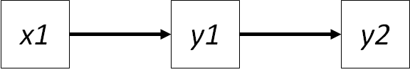
data$y2 <- data$y1 + runif(100)In this case, the path coefficient connecting \(x1 -> y1\) is the regression coefficient \(\gamma_{y1,x1}\). Similarly, the path coefficient connecting \(y1 -> y2\) is the regression coefficient \(\beta_{y2,y1}\). If the data are standardized, then the regression coefficient equals the correlation between the two:
(pathx1_y1 <- summary(lm(y1 ~ x1, as.data.frame(apply(data, 2, scale))))$coefficients[2, 1])## [1] 0.6964617cor(data$y1, data$x1)## [1] 0.6964617(pathy1_y2 <- summary(lm(y2 ~ y1, as.data.frame(apply(data, 2, scale))))$coefficients[2, 1])## [1] 0.6575341cor(data$y2, data$y1)## [1] 0.6575341Note the distinction between exogenous and endogenous linkages, which are represented with \(\gamma\), and relationships between two endogenous variables, which are represented with \(\beta\).
2.2.3 Rule 3: The strength of a compound path (one that includes multiple links) is the product of the individual coefficients.
One of the strengths of SEM is being able to quantify indirect or cascading linkages. This is accomplished by simply multiplying the path coefficients. So the effect of \(x1\) on \(y2\) is the product of the coefficient of the path \(x1 -> y1\) and \(y1 -> y2\):
pathx1_y1 * pathy1_y2## [1] 0.4579473By our earlier logic, this value should equal the correlation between \(x1\) and \(y2\):
cor(data$y2, data$x1)## [1] 0.4484743Ahh, but wait! The correlations are not the same. This result implies that the relationship between \(x1\) and \(y2\) cannot be fully explained by the indirect path through \(y1\). Rather, we require additional information to solve this problem, and it comes in the form of the missing link between \(x1 -> y2\), which we can add to the model:
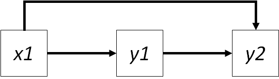
Introducing this path raises a new issue: the relationship between \(y1\) and \(y2\) now arises from two sources. The first is their direct link, the second is the indirect effect of \(x1\) on \(y2\) through \(y1\). We require a new approach to be able to compute the independent effects of each variable on the others, which comes in the form of the ‘partial’ regression coefficient.
2.2.4 Rule 4. When variables are connected by more than one pathway, each pathway is the ‘partial’ regression coefficient.
A partial regression coefficient accounts for the joint influence of more than one variable on the response. In other words, the coefficient for one predictor controls for the influence of other predictors in the model. In this new model, \(y2\) is affected by two variables: \(x1\) and \(y1\).
Procedurally, this involves removing the shared variance between \(x1\) and \(y1\) so that their associations with \(y2\) can be independently derived.
We can calculate the partial effect of \(x1\) through the following equation:
\[b_{y2x1} = \frac{r_{x1y2} - (r_{x1y1} \times r_{y1y2})}{1 - r_{x1y1}^2}\]
which takes the bivariate correlation between \(x1\) and \(y2\), removes the joint influence of \(y1\) and both \(x1\) on \(y2\), then scales this effect by the shared variance between \(x1\) and \(y1\). The result is the partial effect of \(x1\) on \(y2\).
(partialx1 <- (cor(data$x1, data$y2) - (cor(data$x1, data$y1) * cor(data$y1, data$y2))) / (1 - cor(data$x1, data$y1)^2))## [1] -0.0183964It is important to note that partial coefficients implement a statistical (rather than experimental) control. In other words, the partial effect of \(x1\) accounts for the statistical contributions of \(y1\). Thus, partial effects are useful in situations where experimental controls are difficult or impossible to apply.
Notably, we can back out the unstandardized coefficient by multiplying by the ratio of standard deviations of the response over the predictor:
((cor(data$x1, data$y2) - (cor(data$x1, data$y1) * cor(data$y1, data$y2))) / (1 - cor(data$x1, data$y1)^2))* (sd(data$y2)/sd(data$x1))## [1] -0.01754746summary(lm(y2 ~ x1 + y1, data))$coefficients[2, 1]## [1] -0.01754746Similarly, the partial effect of \(y1\) on \(y2\) is given by:
\[b_{y2y1} = \frac{r_{y2y1} - (r_{y2x1} \times r_{y1x1})}{1 - r_{x1y1}^2}\]
(partialy1 <- (cor(data$y2, data$y1) - (cor(data$y2, data$x1) * cor(data$y1, data$x1))) / (1 - cor(data$x1, data$y1)^2))## [1] 0.6703465As before, we can arrive at the same answer by looking at the (standardized) coefficients obtained through multiple regression:
summary(lm(y2 ~ x1 + y1, as.data.frame(apply(data, 2, scale))))$coefficients[2:3, 1]## x1 y1
## -0.0183964 0.6703465partialx1; partialy1## [1] -0.0183964## [1] 0.6703465The regression procedure therefore produces partial coefficients in the case of multiple predictors.
Another way of thinking about this is that the effect of \(x1\) on \(y2\) is computed AFTER having removed the effect of \(y1\) on \(y2\). Procedurally, this can be done by first removing the variance in \(x1\) explained by \(y1\), then regressing the residual values (i.e., the variance in \(y2\) that is unexplained by \(y1\)) against \(y2\).
residsx1 <- residuals(lm(x1 ~ y1, as.data.frame(apply(data, 2, scale))))

summary(lm(scale(data$y2) ~ residsx1))$coefficients[2, 1]
## [1] -0.0183964partialx1## [1] -0.0183964Indeed, this iterative procedure gives us the same value as the former equation based on correlations and the output from the multiple regression.
However, this raises the interesting notion of residual error. The second equation still has variance in \(y2\) that is unassociated with variation in either \(x1\) or \(y1\). In other words, the model does not perfectly predict \(y2\). The idea of residual (unexplained) variance leads us to the fifth rule of path coefficients.
2.2.5 Rule 5: Errors on endogenous variables relate the unexplained correlations or variances arising from unmeasured variables.
Most researchers are familiar with the \(R^2\) statistic, or the ratio of explained variation to the total variation in \(y2\). It follows then that the unexplained or residual variance is \(1 - R^2\).
For example, the error variance on \(y2\) is:
1 - summary(lm(y2 ~ y1 + x1, as.data.frame(apply(data, 2, scale))))$r.squared## [1] 0.5674746This value captures the other (unknown) sources that cause the correlation between \(y2\) and the other variables to deviate from 1. In other words, if \(x1\) is the only variable controlling \(y2\), then their correlation would be 1 and their prediction error would be 0 because we would have accounted for everything that affects \(y2\).
This idea of residual or unexplained variance is easily illustrated with the relationship between \(x1\) and \(y1\) (because there are no partial correlations to deal with), where the square-root of variance explained is simply the correlation coefficient, and 1 - the correlation is the unexplained correlation arising from other sources:
1 - sqrt(summary(lm(y1 ~ x1, as.data.frame(apply(data, 2, scale))))$r.squared)## [1] 0.30353831 - cor(data$y1, data$x1)## [1] 0.3035383In a path diagram, error variances are often represented as \(\zeta\) with an arrow leading into the endogenous variable. The path coefficient representing the effect of \(\zeta\) is often expressed as the error correlation: \(\sqrt(1 - R^2)\), in keeping with the presentation of the other (standardized) coefficients.
2.2.6 Rule 6: Unanalyzed (residual) correlations among two endogenous variables are their partial correlations.
Imagine we remove the path from \(y1 -> y2\):
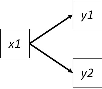
Both variables are endogenous and their relationship can still be quantified, just not in a directed way. If they were exogenous variables, the relationship would be their bivariate correlation (Rule #1), but in this case, we have to remove the effects of \(x1\) on both variables.
\[r_{y1y2\bullet x1} = \frac{r_{y1y2} - (r_{x1y1} \times r_{x1y2})}{\sqrt((1 - r_{x1y1}^2)(1 - r_{x1y2}^2))}\]
This equation removes the effect \(x1\) and scales by the shared variance between \(x1\) and both endogenous variables.
(errory1y2 <- (cor(data$y1, data$y2) - (cor(data$x1, data$y1) * cor(data$x1, data$y2))) / sqrt((1 - cor(data$x1, data$y1)^2) * (1 - cor(data$x1, data$y2)^2)))## [1] 0.5381952As with the partial correlation, this value is the same as the correlation between the residuals of the two models:
(cor(
  resid(lm(y1 ~ x1, as.data.frame(apply(data, 2, scale)))),
  resid(lm(y2 ~ x1, as.data.frame(apply(data, 2, scale))))
))
## [1] 0.5381952errory1y2## [1] 0.5381952Hence these are known as correlated errors and are represented by double-headed arrows between the errors of two endogenous variables. (Often the errors or \(\zeta\)’s are omittedin the diagram, and the graph simply depicts a double-headed arrow between the variables themselves, but the correlation is truly among their errors.)
If the presence of \(x1\) explains all of the variation in \(y1\) and \(y2\), then their partial correlation will be 0. In this case, the two endogenous variables are said to be conditionally independent, or that they are unrelated conditional on the joint influence of \(x1\). If the two are conditionally independent, then the correlation between \(y1\) and \(y2\) is the product of the correlations between \(y1\) and \(x1\), and \(y2\) and \(x1\).
\[r_{y1y2} = r_{y1x1} \times r_{y2x1}\]
(If we replace this term in the previous equation, the numerator becomes 0 and so does the partial correlation.)
Let’s calculate this value:
cor(data$y1, data$x1) * cor(data$y2, data$x1)## [1] 0.3123451Ah, the two are very different, implying that \(y1\) and \(y2\) are not conditionally independent given the joint influence of \(x1\). In other words, there are other, unmeasured sources of variance that are influencing the relationship between these two variables. This interpretation is a good way to think about the notion of correlated errors.
The concept of conditional independence is critical in the implementation of local estimation, principally in the tests of directed separation that form the basis of one goodness-of-fit statistic, which we will revisit in Chapter 3.
Now that we have derived all the quantities related to direct, indirect, and error variances or correlations, we have all the information necessary to calculate total effects.
2.2.7 Rule 7: The total effect one variable has another is the sum of its direct and indirect effects.
If we return to our previous path model, which reinstates the path between \(y1 -> y2\), the total effect of \(x1\) on \(y2\) includes the direct effect as well as the indirect effect mediated by \(y1\).
(totalx1 <- partialx1 + cor(data$y1, data$x1) * partialy1)## [1] 0.4484743This value can be used to demonstrate the final rule.
2.2.8 Rule 8: The total effect (including undirected paths) is equivalent to the total correlation.
We can test this rule easily:
totalx1 == cor(data$y2, data$x1)## [1] TRUEIndeed, the total effect equals the correlation!
If we consider the path model without the directed link between \(y1\) and \(y2\), the correlation between \(y1\) and \(y2\) considers the total effect and undirected effects (i.e., correlated errors between the two endogenous variables):
(totaly1y2 <- cor(data$y1, data$x1) * cor(data$y2, data$x1) + errory1y2 * sqrt(1 - summary(lm(y1 ~ x1, data))$r.squared) * sqrt(1 - summary(lm(y2 ~ x1, data))$r.squared))## [1] 0.6575341totaly1y2 == cor(data$y1, data$y2)## [1] TRUEThis example closes our discussion of path coefficients and their 8 rules.
The major points to remember are:
- standardized coefficients reflect (partial) correlations;
- the indirect effect of one variable on another is obtained by multiplying the individual path coefficients (standardized or unstandardized);
- the total effect is the sum of direct and indirect paths;
- the bivariate correlation is the sum of the total effect plus any undirected paths.
An understanding of covariances and correlations is essential to understanding the solutions provided by a global estimation approach to SEM.
2.3 Variance-based Structural Equation Modeling
The classical approach to SEM is based on the the idea of variance and covariances. With >2 variables, we can construct a variance-covariance matrix, where the diagonals are the variances of each variable and the off-diagonals are the covariances between each pair. Consider our last example:
cov(data)## y1 x1 y2
## y1 0.07602083 0.07970883 0.07178090
## x1 0.07970883 0.17230020 0.07370632
## y2 0.07178090 0.07370632 0.15676481This code returns the variance-covariance matrix for the three variables \(x1\), \(y1\), and \(y2\). We would call this the observed global variance-covariance matrix.
The entire machinery behind covariance-based SEM is to reproduce that global variance-covariance matrix. In fact, all of covariance-based SEM can be boiled down into this simple equation:
\[\Sigma = \Sigma(\Phi)\]
where \(\Sigma\) is the observed variance-covariance matrix, and \(\Sigma(\Phi)\) is the model-estimated covariance matrix expressed in terms of \(\Phi\), the matrix of model-estimated parameters (i.e., coefficients).
In other words, this equation shows that the observed covariances can be understood in terms of statistical parameters that can be used to predict these same covariances. We have already shown that linear regression can be expressed using variances and covariance, and so it follows that covariance-based SEM is simply a multivariate approach to regression.
The question is: how do we arrive at \(\Sigma(\Phi)\), or more relevantly, how do we estimate the matrix of model parameters \(\Phi\) that lead to the estimated variance-covariance matrix?
The most common tool is maximum-likelihood estimation, which iteratively searches parameter space and continually refines estimates of parameter values such that the differences between the observed and expected variance-covariance matrices are minimized.
The maximum-likelihood fitting function can be expressed as:
\[F_{ML} = log|\hat{\Sigma}| + tr(S\hat{\Sigma}^{-1}) - log|S| - (p + q)\]
where \(\Sigma\) is the modeled covariance matrix, \(S\) is the observed covariance matrix, \(p\) is the number of endogenous variables, and \(q\) is the number of exogenous variables. \(tr\) is the trace of the matrix (sum of the diagonal) and the \(^{-1}\) denotes the inverse of the matrix.
Maximum-likelihood estimators have a few desireable properties, principally that they are invariant to the scales of the variables and provide unbiased estimates based on a few assumptions:
- variables must exhibit multivariate normality. Oftentimes this is the not case: dummy variables, interactions and other product terms have non-normal distributions. However, \(F_{ML}\) is fairly robust to violations of multinormality, especially as the sample size grows large.
- the observed matrix \(S\) must be positive-definite. This means there are no negative variances, an implied correlation > 1.0, or redundant variables (one row is a linear function of another).
- finally, \(F_{ML}\) assumes sufficiently large sample size.
The notion of sample size is a good one: as models become increasingly complex, they require more data to fit. The issue of model ‘identifiability’ and sample size is dealt with in the next section.
2.4 Model Identifiability
Like any statistical technique, having sufficient power to test your hypotheses is key to arriving at robust unbiased inferences about your data. This requirement is particularly relevant to SEM, which often evaluates multiple hypotheses simultaneously, and therefore requires more data than other approaches. In this section, we will briefly review the idea of model ‘identifiability’ and sample size requirements.
A model is ‘identified’ if we can uniquely estimate each of its parameters. This not only includes in the matrix of parameter estimates but also their errors. In other words, we need at least as many ‘known’ pieces of information as ‘unknowns’ at minimum to be able to fit a model.
Consider the following equation:
\[a + b = 8\]
We have 1 piece of known information, \(8\), and two unknowns, \(a\) and \(b\). There are a number of solutions for \(a\) and \(b\) (e.g., 1 and 7, 2 and 6, etc), and thus the equation is not solvable. In this case, the model would be underidentified because we lack sufficient information to arrive at a unique solution.
Now consider another equation, in addition to the first:
\[a = 3b\]
With this equation, we now have enough information to uniquely solve for \(a\) and \(b\):
\[(3b) + b = 8\] \[ 4b = 8\] \[b = 8 / 4 = 2\]
\[a + 2 = 8\] \[a = 8 - 2 = 6\]
Thus we have arrived at a single solution for \(a\) and \(b\). We call this system of equations just identified since we have just enough information to solve for the unknowns.
Finally, consider a third equation:
\[2a - 4 = 4b\]
We now have more pieces of known information than unknowns, since we have already arrived at a solution for both \(a\) and \(b\) based on the previous two equations. In this case, we call the system of the equations overidentified because we have more information than is necessary to arrive at unique solutions for our unknown variables. This is the desireable state, because that extra information can be used to provide additional insight, which we will elaborate on shortly.
You may have also heard of models referred to as saturated. Such a model would be just identified; an unsaturated model would be overidentified and and an oversaturated model would be underidentified.
There is a handy rule that can be used to quickly gauge whether a model is under-, just, or overidentified: the “t-rule.” The t-rule takes the following form:
\[t \leq \frac{n(n+1)}{2}\]
where \(t\) is the number of unknowns (parameters to be estimated) and \(n\) is the number of knowns (observed variables). The left hand side is how many pieces of information we want to know. The right hand side reflects the information we have to work with and is equal to the number of unique cells in the observed variance-covariance matrix (diagonal = variance, and lower triangle = covariances).
Consider the simple mediation model from earlier:
In this model, we have several pieces of known information: \(x1\), \(y1\), and \(y2\). So \(n = 3\) for this model.
We need to estimate the parameters related each set of relationships (\(\gamma_{x1y1}\) and \(\beta_{y1y2}\)). These amount to the two covariances, but recall from the first section of this chapter that we need three variances to derive those estimates (\(var_{x1}\), \(var_{y1}\), \(var_{y2}\)). So the total number of unknowns to be estimated is \(t = 5\) (the three variances and the two regression parameters, or covariances).
We can plug in these values to see if we meet the t-rule:
\[5 \leq \frac{3(3+1)}{2} = 6\]
In this case \(5 \leq 6\) holds true and we have enough information to arrive at a unique solution. Note that the right hand side of the equation is the number of entries in the variance-covariance matrix: 3 variances (diagonal) plus 3 covariances (off-diagonal).
Let’s consider our second model, which adds another path:
Now we must additionally estimate the path from \(x1\) to \(y2\) so our value of \(t = 5 + 1\). However, \(6 \leq 6\) and so the t-rule is still satisfied. In this case, however, the model is just identified.
Tallying the number of parameters to be estimated can sometimes be tricky because path diagrams are not always drawn with error variances on the endogenous variables. Additionally, multiple exogenous variables also have a covariance that must be estimated: this is depicted as a non-directional or double-headed error between every pair of exogenous variables. However, these double-headed arrows are rarely drawn, even though they exist. Thus it can be tricky to identify \(n\) in the above equation. In such cases, it is valid to simply count the number of unique cells in the variance-covariance matrix (the diagonal and the lower off-diagonal).
If we were to consider a more complex model, such as one with a feedback from \(y2\) to \(y1\) (in addition to the path from \(y1 -> y2\)) then we would not have enough information to solve the model, which would be underidentified.
Models with bidirectional feedbacks (with separate arrows going in each direction, as opposed to a single double-headed arrow) are referred to as non-recursive. These feedbacks can also occur among variables, for instance: \(x1 -> y1 -> y2 -> x1\) would also be a non-recursive model. Recursive models, then, lack such feedbacks and all causal effects are unidirectional.
Identifiability of non-recursive is tricky. Such models must satisfy the order condition. This condition tests whether variables involved in the feedback have unique information. In our above example of \(y2\) also affecting \(y1\), \(y1\) has unique information in the form of \(x1\) but \(y2\) has no unique information, so it fails the order condition.
The order condition can be evaluated using the following equation:
\[G \leq H\]
where \(G\) = the number of incoming paths, and \(H\) = the number of exogenous variables + the number of indirectly-connected endogenous variabls. In the previous example, \(G = 2\) while \(H = 1\), so the model fails the order condition, as noted.
Model identification is only the first step in determining whether a model can provide unique solutions: sample size can also restrict model fitting by not providing enough replication for the \(F_{ML}\) function to arrive at a stable set of estimates for the path coefficients.
The basic rule-of-thumb is that the level of replication should be at least 5 times the number of estimated coefficients (not error variances or other correlations). So in our previous path model, we are estimating two relationships, so we require at least \(n = 10\) to fit that model.
However, this value is a lower limit: ideally, replication is 5-20x the number of estimated parameters. The larger the sample size, the more precise (unbiased) the estimates will be. This is true for all linear regressions, not just SEM, and so we adopt these guidelines here.
Identifiability and replication are key in not only providing an actual solution, but also in providing extra information with which to evaluate model fit, the topic of the next section.
2.5 Goodness-of-fit Measures
As we have established, the purpose of covariance-based SEM is to reproduce the global observed variance-covariance matrix. However, given that our hypothesized relationships may not actually match the data, we must be prepared to evaluate how well the model-estimated variance-covariance matrix matches the observed variance-covariance matrix.
Recall that in the previous section on Path Coefficients, we evaluated the error variance or correlation as reflecting outside sources of variation uncaptured by our measured variables. High error variances would lead to less accurate estimates of the relationships among variables, and thus a high level of disagreement among the observed and model-implied variance-covariance matrix.
Also recall our formula for the maximum-likelihood fitting function:
\[F_{ML} = log|\hat{\Sigma}| + tr(S\hat{\Sigma}^{-1}) - log|S| - (p + q)\]
where \(\Sigma\) is the modeled covariance matrix, \(S\) is the observed covariance matrix, \(p\) is the number of endogenous variables, and \(q\) is the number of exogenous variables. \(tr\) is the trace of the matrix (sum of the diagonal) and the \(^{-1}\) is the inverse of the matrix.
In the event that \(\Sigma = S\), then the first two terms would equal 0, and similarly for the second two terms. Thus a model where \(F_{ML} = 0\) implies perfect fit because the observed covariance matrix has been exactly reproduced.
Oppositely, a large value of \(F_{ML}\) would imply increasing discrepancy between the observed and model-implied variance-covariance matrices. This could be interpreted as a ‘poor fit’ for the model.
In fact, \(F_{ML}\) is \(\chi^2\)-distributed such that:
\[\chi^2 = (n - 1)F_{ML}\]
which allows us to actually quantify model fit. (In this case \(n\) refers to the sample size.)
We can then formally compare the \(\chi^2\) statistic to the \(\chi^2\)-distribution with some degrees of freedom to achieve a confidence level in the fit. The degrees of freedom are determined by model identification: just identified models will have 0 degrees of freedom (and thus no goodness-of-fit test is possible), and identified models will have \(n(n + 1)/2 - t\) degrees of freedom (where \(n\) are the number of knowns and \(t\) the number of unknowns, from the t-rule).
Failing to reject the null hypothesis that the \(\chi^2\) statistic is different from 0 (the ideal fit) implies a generally good representation of the data (P > 0.05). Alternatively, rejecting the null implies that the \(\chi^2\) statistic is large, as is the discrepancy between the observed and modeled variance-covariance matrices, thus implying a poor fit to the data (P < 0.05). Interpreting the outcome of the significance test is often tricky: unlike testing whether regression parameters are significantly different from zero (something we are all familiar with), in this case, a significant P-value indicates poor fit, so be careful.
The \(\chi^2\) index also provides a way to gauge the relative fit of two models, one of which is nested within the other. The \(\chi^2\) difference test is simply the difference in \(\chi^2\) values between the two models, with the degrees of freedom being the difference in the degrees of freedom between the two models. The resulting statistic can then be compared to a \(\chi^2\) table to yield a significance value. Again, this test is for nested models. For non-nested models, other statistics allow for model comparisons, including AIC and BIC. An AIC or BIC score \(\geq2\) is generally considered to indicate significant differences among models, with smaller values indicating equivalency between the two models.
\(\chi^2\) tests tend to be affected by sample size, with larger samples more likely to generate poor fit due to small absolute deviations (note the scaling of \(F_{ML}\) by \(n-1\) in the above equation). As a result, there are several other fit indices for covariance-based SEM that attempt to correct for this problem:
- Root-mean squared error of approximation (RMSEA): this statistic penalizes models based on sample size. An ‘acceptable’ value is generally <0.10 and a ‘good’ value is anything <0.08.
- Comparative fit index (CFI): this statistic considers the deviation from a ‘null’ model. In most cases, the null estimates all variances but sets the covariances to 0. A value >0.9 is considered good.
- Standardized root-mean squared residual (SRMR): the standardized difference between the observed and predicted correlations. A value <0.08 is considered good.
There are a vast and probably unnecessary number of other fit statistics that have been developed which you may run across. This website has a fairly comprehensive overview, in the event you encounter some of the more uncommon ones in the literature.
What happens if the model doesn’t fit? Depending on the goals of your analysis (e.g., exploratory) you may wish to see which parts of your model have failed to be reproduced by the model-implied variance-covariance matrix. This can be achieved in two ways:
- examination correlation of model residuals: parameters with large residual correlations (difference between observed and expected) could suggest missing information or linkages.
- modification indices, or the expected decrease in the \(\chi^2\) if a missing path were to be included in the model. A high value of a modification index would suggest the missing path should be included. (Tests of directed separation, which we cover in the chapter on Local Estimation, provide similar insight and are returned automatically by piecewiseSEM.)
Users should take caution when exploring these techniques as to avoid dredging the model. SEM is a technique that relies heavily on informed model specification. Adding paths in that are suggested by the data but not anticipated by the user only in an effort to achieve adequate fit might be appropriate in other applications, but ignore the basic philosophy behind SEM that relationships are based on a priori knowledge and intuition.
2.6 Model Fitting Using lavaan
We now have all the pieces necessary to fit an SEM using a covariance-based approach. The package to do so is called lavaan:
library(lavaan)To demonstrate the functionality of this package, let’s use the data from Grace & Keeley (2006), which is included in the piecewiseSEM package:
library(piecewiseSEM)

data(keeley)
In their study, Grace & Keeley wanted to understand patterns in plant diversity following disturbance, in this case wildfires in California.
2.6.1 lavaan vs lm
For purposes of exploration, let’s first consider the relationship between fire severity and stand age (with older stands having more combustible materials).

This is both a linear regression but also a simple SEM, and thus both can be fit using packages in R.
The package to fit the SEM using covariance-based methods is called lavaan (for LAtent VAriable ANalysis, which we will delve into in a later chapter). In lavaan, the syntax is the same as in other modeling functions in R with one key distinction: formulae are passed as character strings. To fit a model in lavaan, it’s first necessary to break down the component models by the endogenous (response) variables and code them as characters. For example:
keeley_formula1 <- 'firesev ~ age'

class(keeley_formula1)
## [1] "character"The function used to fit the model is called (unsurprisingly) sem and accepts the formula string and the dataset:
keeley_sem1 <- sem(keeley_formula1, data = keeley)As with most other models, the function to retrieve the output is summary:
summary(keeley_sem1)## lavaan 0.6-9 ended normally after 11 iterations
##
## Estimator ML
## Optimization method NLMINB
## Number of model parameters 2
##
## Number of observations 90
##
## Model Test User Model:
##
## Test statistic 0.000
## Degrees of freedom 0
##
## Parameter Estimates:
##
## Standard errors Standard
## Information Expected
## Information saturated (h1) model Structured
##
## Regressions:
## Estimate Std.Err z-value P(>|z|)
## firesev ~
## age 0.060 0.012 4.832 0.000
##
## Variances:
## Estimate Std.Err z-value P(>|z|)
## .firesev 2.144 0.320 6.708 0.000The output is organized into a few sections. First is the likelihood optimization method, number of parameters, the total sample size for the model, the estimator (\(F_{ML}\) is the default) and the fit statistic. The model has \(\chi^2 = 0\) with 0 degrees of freedom: this is because we have as many knowns as unknowns, and thus the model is just identified or saturated. To show this, we can apply the t-rule: we must estimate the two variances of the variables plus their path coefficient (\(t = 3\)) and know the values of the two variables (\(n = 2\)). Recall the equation for the t-rule \(t \leq n(n + 1)/2\), so \(3 = 2(2+1)/2 = 6/2 = 3\), and therefore the model is saturated.
Next up are the actual parameter estimates: the relationship between fire severity and stand age is \(\beta = 0.06\) with \(P < 0.001\). The model also reports the estimated error variance on the endogenous variable.
We can dissect this output a little more. First, let’s fit the corresponding linear model using lm:
keeley_mod <- lm(firesev ~ age, data = keeley)

summary(keeley_mod)$coefficients
## Estimate Std. Error t value Pr(>|t|)
## (Intercept) 3.03920623 0.35543253 8.550726 3.448774e-13
## age 0.05967903 0.01249008 4.778113 7.027847e-06You’ll notice that we get the same effect of age on fire severity \(\beta = 0.0596\), but we also get an intercept, which is missing from the previous input. We can force lavaan to return the intercept using the argument meanstructure = T to the sem function:
summary(sem(keeley_formula1, keeley, meanstructure = T))## lavaan 0.6-9 ended normally after 14 iterations
##
## Estimator ML
## Optimization method NLMINB
## Number of model parameters 3
##
## Number of observations 90
##
## Model Test User Model:
##
## Test statistic 0.000
## Degrees of freedom 0
##
## Parameter Estimates:
##
## Standard errors Standard
## Information Expected
## Information saturated (h1) model Structured
##
## Regressions:
## Estimate Std.Err z-value P(>|z|)
## firesev ~
## age 0.060 0.012 4.832 0.000
##
## Intercepts:
## Estimate Std.Err z-value P(>|z|)
## .firesev 3.039 0.351 8.647 0.000
##
## Variances:
## Estimate Std.Err z-value P(>|z|)
## .firesev 2.144 0.320 6.708 0.000which now returns the estimate of the intercept for fire severity. This value is the same as returned by lm.
Returning to our exploration of how path coefficients are calculated, the slope of a simple linear regression is \(b_{xy} = COV_{xy}/VAR_{x}\), which we can recover from the raw data:
cov(keeley[, c("firesev", "age")])[2, 1]/var(keeley$age)## [1] 0.05967903Note that this value is the same returned from both sem and lm. Recall also for simple linear regression that the standardized coefficient is equal to the correlation:
cor(keeley$firesev, keeley$age)## [1] 0.4538654We can obtain the standardized coefficient from lm using the coefs function from piecewiseSEM:
coefs(keeley_mod)## Response Predictor Estimate Std.Error DF Crit.Value P.Value Std.Estimate
## 1 firesev age 0.0597 0.0125 88 4.7781 0 0.4539 ***and indeed, it equals the bivariate correlation!
To return the standardized coefficients using lavaan requires a separate function or another argument. The function is standardizedsolution and returns a table of the standardized coefficients:
standardizedsolution(keeley_sem1)## lhs op rhs est.std se z pvalue ci.lower ci.upper
## 1 firesev ~ age 0.454 0.079 5.726 0 0.299 0.609
## 2 firesev ~~ firesev 0.794 0.072 11.035 0 0.653 0.935
## 3 age ~~ age 1.000 0.000 NA NA 1.000 1.000This output does not return the raw coefficients, however, or any other information about the model that is useful in interpretation. The obtain a single output, you can pass the argument standardize = T to summary:
summary(keeley_sem1, standardize = T)## lavaan 0.6-9 ended normally after 11 iterations
##
## Estimator ML
## Optimization method NLMINB
## Number of model parameters 2
##
## Number of observations 90
##
## Model Test User Model:
##
## Test statistic 0.000
## Degrees of freedom 0
##
## Parameter Estimates:
##
## Standard errors Standard
## Information Expected
## Information saturated (h1) model Structured
##
## Regressions:
## Estimate Std.Err z-value P(>|z|) Std.lv Std.all
## firesev ~
## age 0.060 0.012 4.832 0.000 0.060 0.454
##
## Variances:
## Estimate Std.Err z-value P(>|z|) Std.lv Std.all
## .firesev 2.144 0.320 6.708 0.000 2.144 0.794Now, a few columns are added at the end to report the standardized coefficients.
standardizedsolution also returned the error variance on fire severity, which is \(1 - R^2\). However, lavaan also doesn’t return the \(R^2\) value by default, but can be retrieved using one more argument to summary, rsq = T:
summary(keeley_sem1, standardize = T, rsq = T)## lavaan 0.6-9 ended normally after 11 iterations
##
## Estimator ML
## Optimization method NLMINB
## Number of model parameters 2
##
## Number of observations 90
##
## Model Test User Model:
##
## Test statistic 0.000
## Degrees of freedom 0
##
## Parameter Estimates:
##
## Standard errors Standard
## Information Expected
## Information saturated (h1) model Structured
##
## Regressions:
## Estimate Std.Err z-value P(>|z|) Std.lv Std.all
## firesev ~
## age 0.060 0.012 4.832 0.000 0.060 0.454
##
## Variances:
## Estimate Std.Err z-value P(>|z|) Std.lv Std.all
## .firesev 2.144 0.320 6.708 0.000 2.144 0.794
##
## R-Square:
## Estimate
## firesev 0.206You’ll note that, per Rule 5 of path coefficients, the error variance is \(1 - R^2\).
2.6.2 SEM using lavaan
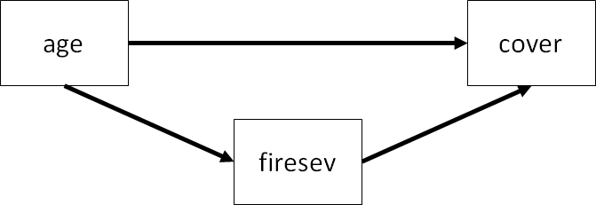
Now that we have covered the basics of lavaan, let’s fit a slightly more complicated SEM. This model is a simplified subset of the full model presented by Grace & Keeley:
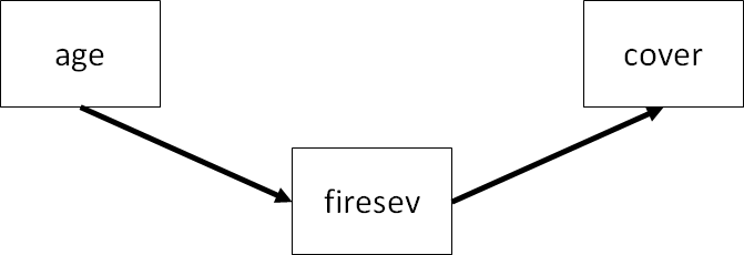
Here, we test the hypotheses that total cover of plants is a function of fire severity, which in turn is informed by how old the plants are in a particular plot (which we have already investigated using linear regression). This test is known as full mediation. In other words, the effect of age is fully mediated by fire severity (we will test another scenario shortly).
Again, we must provide the formulae as a character string. This model can be broken down into two equations (placed on separate lines) representing the two endogenous variables:
keeley_formula2 <- '
firesev ~ age
cover ~ firesev
'
NOTE: Multiple equations will go on separate lines so that lavaan can properly parse the model.
Now let’s fit the SEM and examine the output:
keeley_sem2 <- sem(keeley_formula2, data = keeley)

summary(keeley_sem2, standardize = T, rsq = T)
## lavaan 0.6-9 ended normally after 19 iterations
##
## Estimator ML
## Optimization method NLMINB
## Number of model parameters 4
##
## Number of observations 90
##
## Model Test User Model:
##
## Test statistic 3.297
## Degrees of freedom 1
## P-value (Chi-square) 0.069
##
## Parameter Estimates:
##
## Standard errors Standard
## Information Expected
## Information saturated (h1) model Structured
##
## Regressions:
## Estimate Std.Err z-value P(>|z|) Std.lv Std.all
## firesev ~
## age 0.060 0.012 4.832 0.000 0.060 0.454
## cover ~
## firesev -0.084 0.018 -4.611 0.000 -0.084 -0.437
##
## Variances:
## Estimate Std.Err z-value P(>|z|) Std.lv Std.all
## .firesev 2.144 0.320 6.708 0.000 2.144 0.794
## .cover 0.081 0.012 6.708 0.000 0.081 0.809
##
## R-Square:
## Estimate
## firesev 0.206
## cover 0.191The key difference from our previous application of lavaan is we now have extra information with which to compute the \(\chi^2\) goodness-of-fit statistic. A quick application of the t-rule: unknowns = 3 variances + 2 path coefficients = 5, knowns = 3 variables, so \(5 < 3(3+1)/2 = 6\) leaving us 1 extra degree of freedom.
Moreover, we fail to reject the null that the observed and model-implied variance-covariance matrices are significantly different (\(P = 0.069\)). Thus, we have achieved adequate fit with this model. A note here that the magnitude of the P-value does not reflect increasing fit, only increasing support for the notion that the observed and model-estimated covariances are not different.
Incidentally, we can obtain other fit statistics using the fitMeasures function:
fitMeasures(keeley_sem2)## npar fmin chisq df
## 4.000 0.018 3.297 1.000
## pvalue baseline.chisq baseline.df baseline.pvalue
## 0.069 43.143 3.000 0.000
## cfi tli nnfi rfi
## 0.943 0.828 0.828 0.771
## nfi pnfi ifi rni
## 0.924 0.308 0.945 0.943
## logl unrestricted.logl aic bic
## -176.348 -174.699 360.696 370.695
## ntotal bic2 rmsea rmsea.ci.lower
## 90.000 358.071 0.160 0.000
## rmsea.ci.upper rmsea.pvalue rmr rmr_nomean
## 0.365 0.101 0.245 0.245
## srmr srmr_bentler srmr_bentler_nomean crmr
## 0.062 0.062 0.062 0.088
## crmr_nomean srmr_mplus srmr_mplus_nomean cn_05
## 0.088 0.062 0.062 105.849
## cn_01 gfi agfi pgfi
## 182.093 0.966 0.798 0.161
## mfi ecvi
## 0.987 0.126Woah! We’re certainly not lacking in statistics.
Returning to the summary output, we see the same coefficient for \(firesev ~ age\) and a new estimate for \(cover ~ firesev\). In this case, more severe fires reduce cover (not unexpectedly).
Now that we have multiple linkages, we can also compute the indirect effect of age on cover. Recall from Rule 3 of path coefficients that the indirect effects along a compound path are the product of the individual path coefficients: \(0.454 * -0.437 = -0.198\).
We can obtain this value by modifying the model formula to include these calculations directly. This involves giving a name to the coefficients in the model strings, then adding a new line indicating their product using the operator :=:
keeley_formula2.1 <- '
firesev ~ B1 * age
cover ~ B2 * firesev

indirect := B1 * B2
'

keeley_sem2.1 <- sem(keeley_formula2.1, keeley)

summary(keeley_sem2.1, standardize = T)
## lavaan 0.6-9 ended normally after 19 iterations
##
## Estimator ML
## Optimization method NLMINB
## Number of model parameters 4
##
## Number of observations 90
##
## Model Test User Model:
##
## Test statistic 3.297
## Degrees of freedom 1
## P-value (Chi-square) 0.069
##
## Parameter Estimates:
##
## Standard errors Standard
## Information Expected
## Information saturated (h1) model Structured
##
## Regressions:
## Estimate Std.Err z-value P(>|z|) Std.lv Std.all
## firesev ~
## age (B1) 0.060 0.012 4.832 0.000 0.060 0.454
## cover ~
## firesev (B2) -0.084 0.018 -4.611 0.000 -0.084 -0.437
##
## Variances:
## Estimate Std.Err z-value P(>|z|) Std.lv Std.all
## .firesev 2.144 0.320 6.708 0.000 2.144 0.794
## .cover 0.081 0.012 6.708 0.000 0.081 0.809
##
## Defined Parameters:
## Estimate Std.Err z-value P(>|z|) Std.lv Std.all
## indirect -0.005 0.002 -3.336 0.001 -0.005 -0.198Indeed, the indirect path coefficient is the same as computed above.
Naming coefficients can come in handy when specifying, for example, fixed values for specific purposes (e.g., multigroup modeling).
2.6.3 Testing Alternative Structures using lavaan
There is another possible configuration of these variables which includes a directed path between age and cover:
This type of model tests partial mediation, or the idea that the effect of age is partially mediated by fire severity, but there is still a direct effect between age and cover.
Let’s fit the partial mediation model:
keeley_formula3 <- '
firesev ~ age
cover ~ firesev + age
'

keeley_sem3 <- sem(keeley_formula3, data = keeley)

summary(keeley_sem3, standardize = T)
## lavaan 0.6-9 ended normally after 20 iterations
##
## Estimator ML
## Optimization method NLMINB
## Number of model parameters 5
##
## Number of observations 90
##
## Model Test User Model:
##
## Test statistic 0.000
## Degrees of freedom 0
##
## Parameter Estimates:
##
## Standard errors Standard
## Information Expected
## Information saturated (h1) model Structured
##
## Regressions:
## Estimate Std.Err z-value P(>|z|) Std.lv Std.all
## firesev ~
## age 0.060 0.012 4.832 0.000 0.060 0.454
## cover ~
## firesev -0.067 0.020 -3.353 0.001 -0.067 -0.350
## age -0.005 0.003 -1.833 0.067 -0.005 -0.191
##
## Variances:
## Estimate Std.Err z-value P(>|z|) Std.lv Std.all
## .firesev 2.144 0.320 6.708 0.000 2.144 0.794
## .cover 0.078 0.012 6.708 0.000 0.078 0.780Ah, we have a problem: the model is saturated, so there are no degrees of freedom leftover with which to test model fit.
We can, however, use the \(\chi^2\) test to determine whether this model is more or less supported than the partial mediation model, which is called using the function anova:
anova(keeley_sem2, keeley_sem3)## Chi-Squared Difference Test
##
## Df AIC BIC Chisq Chisq diff Df diff Pr(>Chisq)
## keeley_sem3 0 359.4 371.9 0.0000
## keeley_sem2 1 360.7 370.7 3.2974 3.2974 1 0.06939 .
## ---
## Signif. codes: 0 '***' 0.001 '**' 0.01 '*' 0.05 '.' 0.1 ' ' 1(Note that the \(\chi^2\) statistic and associated degrees of freedom are still 0 for the model testing partial mediation.)
We can see from this output that we fail to reject the null that the models are significantly different (\(P = 0.069\)). Because these are nested models, it is also fair to compare them using AIC/BIC. In both cases, the models are deemed equivalent and the more parsimonious model (full mediation) would be preferred. Moreover, examining the output of the model of partial mediation reveals a non-significant effect of age on cover (\(P = 0.067\)). Together, these pieces of information would suggest that plant cover is not directly affected by stand age, but rather the effect of age is entirely mediated through the severity of burns.
2.7 References
Grace, J. B., & Keeley, J. E. (2006). A structural equation model analysis of postfire plant diversity in California shrublands. Ecological Applications, 16(2), 503-514.