7 Latent Variable Modeling
7.1 Introduction to Latent Variable Modeling
Latent variables are variables that are unobserved, but whose influence can be summarized through one or more indicator variables. They are useful for capturing complex or conceptual properties of a system that are difficult to quantify or measure directly. Early applications of latent variables, for example, focused on modeling the effects of ‘general intelligence,’ which is an abstract concept that is impossible to actually measure, but that can be approximated using scores from different tests of cognitive performance (e.g., memory, verbal, spatial, etc.).
Consider the following simple example of a latent variable \(\xi\), in this case exogenous and informed only by a single predictor \(x\):
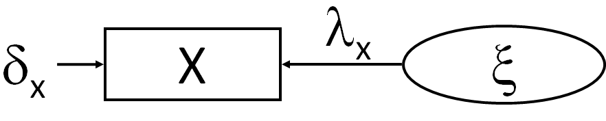
Here, the latent variable is indicated by the circle and the single indicator variable \(x\) is indicated by the square box, as are all observed variables. You’ll note a few curiosities compared to observed-variable models.
First, the direction of causality is reversed from what you might expect: from the latent variables to the observed variable. This is because the indicator variable is an emergent manifestation of the underlying phenomenon represented by the latent variable.
Second, there is an error \(\delta\) associated with the indicator. This implies that the indicator is often an imperfect approximation of the latent construct. In other words, there are presumably other factors influencing the correlation between the observed and latent variable.
The latent variable can be related to the indicator variable using the following equation:
\[x = \lambda \xi + \delta_{x}\]
Here, the values of \(x\) are the result of the latent variable proportional to \(\lambda\) (its effect on \(x\)) plus some error \(\delta_{x}\).
A simple example of a latent-indicator relationship would be body size (latent) and body mass (indicator). There are obviously many aspects to body size that may be difficult to quantify, such as shape, volume, relief, and so on. Body mass is a simple, measurable consequence of these unmeasured characteristics, and thus can be thought to latently indicate the concept of size. However, because we often can’t perfectly measure body mass of every individual in the population in which we are interested, we must incorporate sampling error into our model of body size, indicated by the \(\delta_{x}\).
This example reinforces the point that latent variables are used to represent concepts. Body size is often invoked in lots of ecological hypotheses (e.g., metabolic theory, Bergmann’s rule), but is almost always represented as some easily measurable quantity such as body mass rather than the complex, multidimensional construct that it is in reality. Latent variable modeling allows us to better approach that multidimensional construct by modeling a series of indicator variables that arise from the general concept of body size (e.g., mass, length, width, etc.). It therefore is a powerful tool that is better positioned to integrate theory and observation than relying on one or few surrogates.
However, some care should be taken when constructing latent variables. Just because we call a latent variable something does not always mean it is that thing. For example, the latent variable body size as indicated by total abundance might appear legitimate–high abundances may constrain body sizes under limited resources–but is abundance really an indicator of this phenomenon? Can we go on to evaluate ecological theory about metabolic scaling on the basis of abundances? Kind of a stretch. So care should be taken when selecting or naming latent variables and identifying appropriate indicators (known as the naming fallacy). In other words: be sure the latent variable reflects the actual properties captured by the indicator variables! The degree to which the indicators represent the phenomenon captured by the latent variable is termed validity and is a qualitative justification of the latent construct.
In contrast, the reliability of the latent variable captures how well an indicator reflects the latent variable through a quantitative value. High reliability implies that the same values of the indicator would be obtained if they were continually resampled again and again. In other words, reliable indicators approach the true population mean that is the (theoretical) product of the latent variable: a perfect indicator would yield the same values every time so they would all have a correlation \(r = 1\). Of course, rarely do we sample an entire population so well or so exhaustively, and there will inevitably be some differences among our samples leading to deviations in \(r\) away from 1.
From the actual observed correlation among repeated measures of \(x\), we can obtain a path coefficient from the latent variable to the indicator. Recall from the fifth rule of path coefficients that the coefficient on the path from the error variance \(\zeta\) is the square-root of the unexplained variance. In this case, we want the opposite: we want the shared variance between the latent and indicator variable (a lot of shared variance is what makes a good indicator!). As in the case of the error path, the path coefficient from the latent variable to the indicator is often expressed in its standardized form: the square-root of the reliability. This value is also called the loading.
From the reliability, we can also obtain the standardized error term \(\delta_{x}\). This is the unshared variance, or 1 - the reliability. For the unstandardized form, one can apply the following equation:
\[\delta_{x} = (1 - \lambda_{x}^2) \times VAR_{x}\]
As with other coefficients, standardization is applied simply because multiple indicators may be measured in vastly different units, and one may wish to fairly compare the loadings and errors.
Let’s construct a simple example. Say we sample the variable \(x\) repeatedly 5 times with \(n = 10\). This could be 5 sampling dates or 5 separate trials.
set.seed(11)

x <- rnorm(10)

x.list <- lapply(1:5, function(i) x + runif(10, 0, 2))

x. <- unlist(x.list)
We can compute the average correlation among all trials. This is our measure of reliability:
combos <- combn(1:5, 2)

cors <- c()

for(i in 1:ncol(combos)) cors <- c(cors, cor(x.list[[combos[1, i]]], x.list[[combos[2, i]]]))

(r <- mean(cors))
## [1] 0.804403From this value \(r = 0.804\), we can obtain the path coefficient and the (standardized) error variance:
sqrt(r) # path coefficient## [1] 0.89688521 - r # standardized error variance## [1] 0.195597(1 - r) * var(unlist(x.list)) # unstandardized error variance## [1] 0.213149In summary: the standardized coefficient (the loading) linking indicator to latent variables is the square-root of the reliability. The standardized error variance is 1 - reliability.
So far, we have only dealt with latent variables as exogenous (predictor) variables, but they can also act as endogenous (response) variables. Here is an example endogenous latent variable:
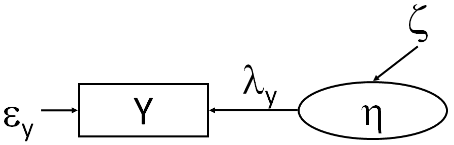
The graph looks roughly similar, with some changes in the parameters: the error variance on \(y\) is now \(\epsilon_{y}\), while the latent variable itself is represented as \(\eta\) and it has its own error \(\zeta\). The presence of this additional error presents a challenge: we simply don’t have enough information to estimate all the unknowns here.
In this case, we assume no measurement error on \(y\) such that \(\epsilon_{y} = 0\). Consequently, \(y\) becomes a perfect indicator of \(\eta\) such that the reliability is total and \(\lambda_{y} = 1\). We will get the calculation of \(\zeta\) now because this involves the values of one or more paths leading into the endogenous \(\eta\).
7.2 Application of Latent Variables to Path Models
Having now described both exogenous and endogenous latent variables now allows us to fit a structural model, or one with directed paths between latent variables. This is in contrast to a measurement model, which focuses solely on relating indicators to latent variables.
As an example of a structural model, let’s combine the two latent variable models so that the exogenous latent variable is predicting the endogenous one:
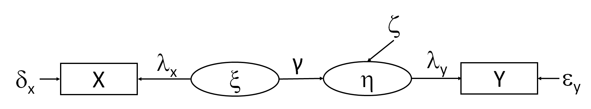
As before, let’s fix the error of \(y\) to be 0 so that the loading on \(\eta = 1\). We can solve the exogenous paths as before, leaving us with two parameters left: the path coefficient \(\gamma\) and \(\zeta\).
We can solve the path coefficient \(\gamma\) by knowing the regression coefficient (correlation) between the raw values of \(x\) and \(y\) and adjusting by the loading of \(x\) on \(\xi\).
Let’s return to our previous example and generate some data for \(y\), then estimate the standardized coefficient or correlation:
set.seed(3)

y <- x + runif(10, 0, 5)

y.list <- lapply(1:5, function(i) y + runif(10, 0, 2))

y. <- unlist(y.list)

xy_model <- lm(y. ~ x.)

beta <- summary(xy_model)$coefficients[2, 1]

(beta_std <- beta * (sd(x.) / sd(y.))) # standardized
## [1] 0.5440115cor(x., y.) # same as the standardized coefficient for simple regression## [1] 0.5440115In this example, the estimated standardized path coefficient for \(x\) on \(y\) is \(b = 0.544\).
We can obtain an estimate of gamma using the following equation:
\[\gamma = \frac{b}{\lambda_{x}}\]
Which, for our example, is:
(gamma <- beta_std / sqrt(r))## [1] 0.6065565So the new estimate of the coefficient between the two latent variables is \(\gamma = 0.607\) which of course is different from \(b = 0.544\). This is because the measurement error in \(x\) was formerly lumped in to the prediction error of \(y\). By removing it, we have improved the estimate of the true effect of \(x\) on \(y\) and validated our assumption about the error variance of \(y\). Not accounting for measurement error, then, results in a downward bias in both the coefficients and the variance explained.
From this value, we can obtain the unexplained variance, or \(\zeta\). Recall that the error \(\delta_{x}\) is 1 - the explained variance, where the explained variance is the reliability. Here, we can transfer this knowledge such that: \(\zeta = 1 - \gamma^2\):
1 - gamma^2## [1] 0.6320892# compare to regression residual variance
1 - summary(xy_model)$r.squared## [1] 0.7040515The error variance has decreased from 0.704 to 0.632 relative to the linear model, again, as a consequence of removing the measurement error in \(x\) in the predictions of \(y\) and improving our estimate of the true relationship between the two.
7.3 Latent Variables in lavaan
Let’s reproduce this example using lavaan. The setup is almost identical except for a new operator =~ which indicates a latent variable. Additionally, we will fix the error variance in \(x\) to the known (unstandardized) error variance from our repeated trials (recall how to fix coefficients from the chapter on multigroup models).
library(lavaan)

(1 - r) * var(x.) # unstandardized error variance
## [1] 0.213149latent_formula1 <- '
xi =~ x # exogenous latent
eta =~ y # endogenous latent
eta ~ xi # path model
x ~~ 0.213 * x # fix error variance
'
latent_model1 <- sem(latent_formula1, data.frame(x = x., y = y.))
summary(latent_model1, standardize = T, rsq = T)## lavaan 0.6-9 ended normally after 22 iterations
##
## Estimator ML
## Optimization method NLMINB
## Number of model parameters 3
##
## Number of observations 50
##
## Model Test User Model:
##
## Test statistic 0.000
## Degrees of freedom 0
##
## Parameter Estimates:
##
## Standard errors Standard
## Information Expected
## Information saturated (h1) model Structured
##
## Latent Variables:
## Estimate Std.Err z-value P(>|z|) Std.lv Std.all
## xi =~
## x 1.000 0.925 0.895
## eta =~
## y 1.000 1.504 1.000
##
## Regressions:
## Estimate Std.Err z-value P(>|z|) Std.lv Std.all
## eta ~
## xi 0.989 0.221 4.469 0.000 0.608 0.608
##
## Variances:
## Estimate Std.Err z-value P(>|z|) Std.lv Std.all
## .x 0.213 0.213 0.199
## .y 0.000 0.000 0.000
## xi 0.855 0.214 4.003 0.000 1.000 1.000
## .eta 1.426 0.327 4.363 0.000 0.630 0.630
##
## R-Square:
## Estimate
## x 0.801
## y 1.000
## eta 0.370If we examine the output, we find a poor-fitting model, but let’s ignore that for now considering these were just random data. Instead, let’s focus on the estimated parameters and compare them to our hand-calculated values.
The standardized loading on \(xi = 0.895\) which is very close to the value we calculated \(\sqrt(r) = 0.897\). The loading on \(\eta\) is \(\lambda_{y} = 1\). Notice how we didn’t specify that: the default in lavaan is to set the first loading to 1 when the error variance is not supplied (more on this later).
With respect to the regression coefficient, lavaan returned a standardized \(\gamma = 0.608\) while we obtained \(\gamma = 0.607\). Very close! Similarly the standardized error variance on \(\eta\) is \(\zeta = 0.630\), which is also very close to \(1 - \gamma^2 = 0.632\). Naturally, then, the explained variances are also nearly identical, being 1 - error variance.
So, all in all, for single indicator latent variables, we are able to almost exactly reproduce the output from lavaan (slight deviations are due to the optimization algorithms to solve the maximum-likelihood fitting function).
One could alternately fix the error of the exogenous latent variable and incorporate measurement error of \(y\):
cors.y <- c()

for(i in 1:ncol(combos)) cors.y <- c(cors.y, cor(y.list[[combos[1, i]]], y.list[[combos[2, i]]]))

(r.y <- mean(cors.y))
## [1] 0.8535083(1 - r.y) * var(y.) # unstandardized error variance## [1] 0.3380926latent_formula2 <- '
xi =~ x # exogenous latent
eta =~ y # endogenous latent
eta ~ xi # path model
y ~~ 0.338 * y # fix error variance
'
latent_model2 <- sem(latent_formula2, data.frame(x = x., y = y.))
summary(latent_model2, standardize = T, rsq = T)## lavaan 0.6-9 ended normally after 11 iterations
##
## Estimator ML
## Optimization method NLMINB
## Number of model parameters 3
##
## Number of observations 50
##
## Model Test User Model:
##
## Test statistic 0.000
## Degrees of freedom 0
##
## Parameter Estimates:
##
## Standard errors Standard
## Information Expected
## Information saturated (h1) model Structured
##
## Latent Variables:
## Estimate Std.Err z-value P(>|z|) Std.lv Std.all
## xi =~
## x 1.000 1.033 1.000
## eta =~
## y 1.000 1.387 0.922
##
## Regressions:
## Estimate Std.Err z-value P(>|z|) Std.lv Std.all
## eta ~
## xi 0.792 0.173 4.584 0.000 0.590 0.590
##
## Variances:
## Estimate Std.Err z-value P(>|z|) Std.lv Std.all
## .y 0.338 0.338 0.149
## .x 0.000 0.000 0.000
## xi 1.068 0.214 5.000 0.000 1.000 1.000
## .eta 1.254 0.318 3.939 0.000 0.652 0.652
##
## R-Square:
## Estimate
## y 0.851
## x 1.000
## eta 0.348Here, because we did not specify it, the error variance of \(x\) has automatically been fixed to 0 and the loading to 1, again, because we have more unknowns than knowns and have to sacrifice a value to get estimates for everything else.
To start, the standardized \(\gamma = 0.590\), which is different than the \(\gamma = 0.608\) we obtained when incorporating measurement error on \(x\), but also different than the standardized coefficient from a simple linear regression \(b = 0.544\).
The error variance on \(\eta\) (\(\zeta = 0.652\)) is also lower than the unexplained variance from the linear regression (\(1 - R^2 = 0.704\)), but higher than in the latent variable model incorporating error on \(x\) (\(\zeta = 0.630\)).
Thus, we see that incorporating measurement error in endogenous latent variables resolves some of the downward bias in the unstandardized coefficient and error variance.
For the moment, latent variables are restricted to covariance-based SEM, although new work by Shipley and Douma have extended latent variable modeling to a graph theoretic approachk. For the time being, however, lavaan provides an easier, robust framework that easily extends to multi-indicator latent variables, and so we will use it from here on out.
7.4 Multi-indicator Latent Variables
Accounting for measurement error requires some estimate of reliability. Often, we don’t have a measure of reliability, because we don’t design our experiments to repeatedly sample the indicator variable to obtain one. In such cases, it might be recommended to revert to a non-latent variable approach where the path coefficients are simlpy regression coefficients that don’t incorporate any measurement error.
Another solution is to incorporate multiple indicator variables to provide a different measure of reliability. In this case, the correlation is not derived from multiple samples of the same indicator, but among indicators. It also acts as a check against indicators that do not inform the latent variable, as such variables will provide low reliability estimates because they are (presumably) not being generated by that same underlying latent variable.
This approach also provides a conceptual advantage: we often choose a single indicator as a surrogate for a latent concept (e.g., body mass for body size). Including more indicators helps to generalize this phenomenon by testing that the result is not an impact of the choice of any single indicator.
Multiple indicators raises a new problem, though: identifiability. Remember from the chapter on global estimation that we must have enough known pieces of information to estimate all the unknown quantities implied by the model. Latent variable models must also follow the “t-rule.”
Consider an exogenous latent variable indicated by two variables, \(x1\) and \(x2\). We can break this latent variable into two equations:
\[x1 = \lambda_{1}\xi + \delta_{x1}\] \[x2 = \lambda_{2}\xi + \delta_{x2}\]
We know the values of \(x1\) and \(x2\) and the correlation between them. To estimate values for the latent construct \(\xi\) we need to estimate \(\lambda_{1}\), \(\lambda_{2}\), \(\delta_{x1}\) and \(\delta_{x2}\). This model fails the t-rule, which, if you recall, is:
\[t \leq \frac{n(n+1)}{2}\]
where \(t = 4\) is the number of unknowns, and \(n = 2\) is the number of knowns. In this example, \(t = 4 \leq 3\) does not hold.
Since \(\delta = 1 - \lambda^2\), we need only solve for the two \(\lambda\)s, but we only have one piece of information: the correlation. The solution is to set the loadings to be equal: \(\lambda_{1} = \lambda_{2}\). This is because, with only this information, we have no reason to suspect one indicator is more correlated with the latent variable than the other. Its important to note here that the two must be positively correlated (or scaled to be so), otherwise setting them to be equal is not a valid assumption.
We know from our “ninth rule of path coefficients” that the correlation equals the sum of the direct and indirect pathways. The only path connecting \(x1\) and \(x2\) is through \(\epsilon\), and the value of the compound path is the product of the two individual pathways (Rule 3). Thus, the correlation \(r_{x1,x2} = \lambda_{1} \times \lambda_{2}\). Given the assumption that the two loadings are equal, \(r_{x1,x2} = \lambda^2\) and thus \(\lambda = \sqrt(r_{x1,x2})\).
We can scale this procedure for >2 indicators by setting just the two loadings to be equal: this will give us the necessary information (along with Rule 8 of path coefficients) to generate unique solutions for the other loadings. It is for this reason that at least three indicators are preferred for multi-indicator latent variables: it lessens the impact of the assumption that two of the loadings are equal.
A potentially better–and easier–solution is to fix one of the loadings to be 1. If, for example, we fix \(\lambda_{1} = 1\) then we know that \(\lambda_{2} = r_{x1,x2} / \lambda_{1} = r_{x1,x2} / 1 = r_{x1,x2}\).
This choice has another consequence: because it is unmeasured, we also need to provide a scale for our multi-indicator latent variable. This can be done by fixing the variance \(\zeta = 1\) or by fixing one of the unstandardized loadings to 1 (wherein the scale will be in units of that indicator). Both accomplish the same objective.
Finally, we can obtain an integrated estimate of reliability from multi-indicator latent variables using the following equation:
\[\rho = \frac{(\sum\lambda_{j})^2}{(\sum\lambda_{j})^2 + \sum\epsilon_{j}} \]
where \(j\) is the index of each indicator variable.
For the record, a reliability index > 0.9 is considered ‘excellent’, > 0.8 to be ‘good’, and so on. Anything < 0.5 is considered to be no different than random chance, and so indicators with such a low degree of correlation should be avoided.
In fact, it is always recommended to inspect the correlation matrix among indicator variables to screen for potentially unrelated indicators. It may also help to identify indicators that are highly correlated, moreso than the other indicators. Such high correlations might suggest another common cause (such as the same measurement instrument, same observer, evolutionary constraints, etc.). In this case, it would be recommended to indicate a ‘correlated error’ among the two indicators indicating a separate underlying driver of their higher-than-average association than the specified latent construct.
When we get into the realm of multi-indicator latent variables, it becomes impossible to decompose partial relationships as we have previously for observed variable models. Instead, maximum-likelihood functions are necessary to iteratively test and optimize the parameters that describe the relationships between observed and unobserved quantities.
As in observed-variable models, the maximum-likelihood fitting function (\(F_{ML}\)) can be used to construct a \(\chi^2\) statistic that is the difference between the observed and model-implied variance-covariance matrices. In the case of latent variable models, the covariances among latent variables as well as the loadings are considered in constructing the estimated covariance matrix. Beyond that, the procedure is the same as for observed variable models in terms of calculating \(\chi^2\) and testing it against the \(\chi^2\)-distribution with some model degrees of freedom.
7.5 Confirmatory Factor Analysis
Multi-indicator latent variables can also be used to the test the hypothesis that a suite of indicator variables are generated by the same underlying process. This is also called confirmatory factor analysis. In other words, you are testing the idea that the latent variable has given rise to emergent properties that, by virtue of a common cause, are correlated. This approach concerns only the measurement model and thus is a precursor to evaluation of any structural models in which the latent variables appear.
In contrast, exploratory factor analysis assumes that all latent variables are indicated by all observed variables.
[content pending]
7.6 Travis & Grace (2010): An Example
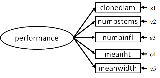
Let’s apply these concepts to an example dataset from Travis & Grace (2010). In this example, the authors transplanted individuals of the salt marsh plant Spartina alterniflora and measured their performance relative to local populations. In this case, performance was captured by a number of variables including: stem density, the number of infloresences, clone diameter, leaf height, and leaf width. The difference between transplants and local individuals was quantified using their genetic dissimilarity.
In this case, the authors considered ‘performance’ to be a latent construct that manifests in the five indicators listed above:
Let’s first explore this latent construct before getting into the structural model. First, let’s examine the raw correlations to see if this construct is justifiable:
travis <- read.csv("https://raw.githubusercontent.com/jslefche/sem_book/master/data/travis.csv")

cor(travis[, 4:8])
## stems infls clonediam leafht leafwdth
## stems 1.0000000 0.8339227 0.9333150 0.7275625 0.6457378
## infls 0.8339227 1.0000000 0.8126388 0.6925888 0.6026302
## clonediam 0.9333150 0.8126388 1.0000000 0.7729843 0.7296621
## leafht 0.7275625 0.6925888 0.7729843 1.0000000 0.9687725
## leafwdth 0.6457378 0.6026302 0.7296621 0.9687725 1.0000000The correlations range from 0.65-0.93, suggesting that many of these variables may be generated by the same process. There is one excessive correlation between leaf height and width, potentially suggesting influence by another process (hint hint).
Now that we have qualitatively assessed the validity of the latent model, let’s fit it and examine the output:
travis_latent_formula1 <- 'performance =~ stems + infls + clonediam + leafht + leafwdth'

travis_latent_model1 <- sem(travis_latent_formula1, travis)
## Warning in lav_object_post_check(object): lavaan WARNING: some estimated ov
## variances are negativesummary(travis_latent_model1)## lavaan 0.6-9 ended normally after 82 iterations
##
## Estimator ML
## Optimization method NLMINB
## Number of model parameters 10
##
## Number of observations 23
##
## Model Test User Model:
##
## Test statistic 51.106
## Degrees of freedom 5
## P-value (Chi-square) 0.000
##
## Parameter Estimates:
##
## Standard errors Standard
## Information Expected
## Information saturated (h1) model Structured
##
## Latent Variables:
## Estimate Std.Err z-value P(>|z|)
## performance =~
## stems 1.000
## infls 0.126 0.037 3.377 0.001
## clonediam 1.160 0.309 3.751 0.000
## leafht 1.215 0.244 4.971 0.000
## leafwdth 0.151 0.031 4.822 0.000
##
## Variances:
## Estimate Std.Err z-value P(>|z|)
## .stems 125.886 37.014 3.401 0.001
## .infls 2.405 0.707 3.403 0.001
## .clonediam 132.478 39.038 3.394 0.001
## .leafht -1.847 5.336 -0.346 0.729
## .leafwdth 0.223 0.105 2.131 0.033
## performance 135.763 67.580 2.009 0.045Note that the first loading has been restricted to 1 (the default in lavaan) for purposes of identifiability.
First, we note that the model is a poor fit (P < 0.001). We can explore why this is using modification indices:
print(modindices(travis_latent_model1))## lhs op rhs mi epc sepc.lv sepc.all sepc.nox
## 12 stems ~~ infls 10.470 11.784 11.784 0.677 0.677
## 13 stems ~~ clonediam 17.152 112.521 112.521 0.871 0.871
## 14 stems ~~ leafht 0.693 -7.889 -7.889 -0.517 -0.517
## 15 stems ~~ leafwdth 2.214 -1.836 -1.836 -0.346 -0.346
## 16 infls ~~ clonediam 8.773 11.092 11.092 0.621 0.621
## 17 infls ~~ leafht 0.062 -0.312 -0.312 -0.148 -0.148
## 18 infls ~~ leafwdth 2.906 -0.281 -0.281 -0.383 -0.383
## 19 clonediam ~~ leafht 4.028 -21.233 -21.233 -1.357 -1.357
## 20 clonediam ~~ leafwdth 0.037 -0.261 -0.261 -0.048 -0.048
## 21 leafht ~~ leafwdth 37.862 17.177 17.177 26.752 26.752Recall that the value of the modification index (mi in the output) is the expected decrease in the model \(\chi^2\). Here, a larger number would lead to a better fit if that path were included. It seems there is a strong implied correlation between leaf height and leaf width, presumably arising from common constraints on how the leaves of Spartina have evolved and the limited variety of shapes they can take, and not from the plant’s performance.
We can introduce this correlation into the model and re-fit:
travis_latent_formula2 <- '
performance =~ stems + infls + clonediam + leafht + leafwdth
leafht ~~ leafwdth
'

travis_latent_model2 <- sem(travis_latent_formula2, travis)

summary(travis_latent_model2)
## lavaan 0.6-9 ended normally after 81 iterations
##
## Estimator ML
## Optimization method NLMINB
## Number of model parameters 11
##
## Number of observations 23
##
## Model Test User Model:
##
## Test statistic 7.410
## Degrees of freedom 4
## P-value (Chi-square) 0.116
##
## Parameter Estimates:
##
## Standard errors Standard
## Information Expected
## Information saturated (h1) model Structured
##
## Latent Variables:
## Estimate Std.Err z-value P(>|z|)
## performance =~
## stems 1.000
## infls 0.117 0.016 7.173 0.000
## clonediam 1.086 0.096 11.319 0.000
## leafht 0.697 0.127 5.509 0.000
## leafwdth 0.082 0.018 4.529 0.000
##
## Covariances:
## Estimate Std.Err z-value P(>|z|)
## .leafht ~~
## .leafwdth 10.831 3.432 3.156 0.002
##
## Variances:
## Estimate Std.Err z-value P(>|z|)
## .stems 15.267 10.877 1.404 0.160
## .infls 1.204 0.390 3.085 0.002
## .clonediam 24.786 13.830 1.792 0.073
## .leafht 78.958 24.465 3.227 0.001
## .leafwdth 1.672 0.509 3.283 0.001
## performance 246.382 77.658 3.173 0.002Ah-ha! Introducing this correlated error has now reduced the \(\chi^2\) statistic to an acceptably low level to achieve an adequate model fit (P = 0.116). Thus, we fail to reject our latent construct of plant performance, which we can now use to evaluate some broader hypotheses.
If you recall, the authors’ original intent was to explore how native vs. non-native genotypes of Spartina influenced performance, which they quantified using a measure of genetic distance from the local population. To test this hypothesis, let’s fit the following path model:
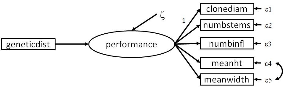
Let’s fit the above model:
travis_path_formula1 <- '
# latent
performance =~ stems + infls + clonediam + leafht + leafwdth

# structural paths
performance ~ geneticdist

# correlated errors
leafht ~~ leafwdth
'

travis_path_model1 <- sem(travis_path_formula1, travis)

summary(travis_path_model1)
## lavaan 0.6-9 ended normally after 107 iterations
##
## Estimator ML
## Optimization method NLMINB
## Number of model parameters 12
##
## Number of observations 23
##
## Model Test User Model:
##
## Test statistic 12.237
## Degrees of freedom 8
## P-value (Chi-square) 0.141
##
## Parameter Estimates:
##
## Standard errors Standard
## Information Expected
## Information saturated (h1) model Structured
##
## Latent Variables:
## Estimate Std.Err z-value P(>|z|)
## performance =~
## stems 1.000
## infls 0.117 0.017 6.929 0.000
## clonediam 1.106 0.096 11.508 0.000
## leafht 0.711 0.127 5.601 0.000
## leafwdth 0.084 0.018 4.650 0.000
##
## Regressions:
## Estimate Std.Err z-value P(>|z|)
## performance ~
## geneticdist -51.673 11.365 -4.547 0.000
##
## Covariances:
## Estimate Std.Err z-value P(>|z|)
## .leafht ~~
## .leafwdth 10.416 3.312 3.145 0.002
##
## Variances:
## Estimate Std.Err z-value P(>|z|)
## .stems 19.691 10.733 1.835 0.067
## .infls 1.246 0.401 3.108 0.002
## .clonediam 19.411 12.364 1.570 0.116
## .leafht 76.177 23.645 3.222 0.001
## .leafwdth 1.612 0.492 3.278 0.001
## .performance 120.509 39.656 3.039 0.002It seems that this model fits the data well (P = 0.141) and the relationship of interest (between \(geneticdist\) and \(performance\)) is highly significant (P < 0.001). In this case, the more distant the genotypes of the local population from which the transplants were taken (i.e., a greater genetic distance), the worse they performed.
7.7 References
Travis, S. E., & Grace, J. B. (2010). Predicting performance for ecological restoration: a case study using Spartina alterniflora. Ecological Applications, 20(1), 192-204.