5 Categorical Variables
While SEM was initially derived to consider only continuous variables (and indeed most applications still do), it’s often the case–especially in ecology–that the observed variables are discrete. For example: binary (yes/no, failure/success, etc.), nominal (site 1, site 2), or ordinal levels (small < medium < large). Newer advances in modeling allow for the incorporation, either directly or in a more roundabout fashion, of categorical variables into SEM.
There are two way that categorical variables could be included: as exogenous (predictors) or endogenous (responses). We will deal with the simpler case of exogenous categorical variables first, as they pose not so much of a computational issue but a conceptual one.
5.1 Introduction to Exogenous Categorical Variables
Recall that a linear regression predicting y has the following standard form:
\[y = \alpha + \beta_{1}*x_{1} + \epsilon\]
where \(\alpha\) is the intercept, \(\beta_{1}\) is the slope of the effect of \(x\) on y, and \(\epsilon\) is the residual error.
When \(x\) is continuous, the intercept \(\alpha\) is intepreted as the value of y when \(x\) = 0. All good.
For categorical factors, the intercept \(\alpha\) has a different interpretation. Consider a value of \(x\) with \(k\) levels. Since the levels of \(x\) are discrete and presumably can never assume a value of 0, \(\alpha\) is instead the mean value of y at the ‘reference’ level of \(x\). (In R, the reference level is the first level alphabetically, although this can be reset manually.) The regression coefficients \(\beta_{k}\) are therefore the effect of each other level relative to the reference level. So for \(k\) levels, there are \(k - 1\) coefficients estimated with the additional \(\alpha\) term reflecting the \(k\)th level.
Another way to think about this phenomenon is using so-called ‘dummy’ variables. Imagine each level was broken into a separate variable with a value of 0 or 1: a two-level factor with levels “a” and “b” would then become two factors “a” and “b” each with the levels 0 or 1. (In R, this would mean transposing rows as columns.)
Now imagine setting all the values of these dummy variables to 0 to estimate the intercept: this would imply the total absence of the factor, which is not a state. Another way of thinking about this is that the dummy variables are linearly dependent: if “a = 1” then by definition “b = 0” as the response variable cannot occupy the two states simultaneously. Hence the need to set one level as the reference, so that the effect of “a” can be interpreted relative to the absence of “b”, and also why you don’t recover as many coefficients as there are levels. I once heard it state that one level had to “fall on the sword” so that we can estimate the other levels.
This behavior presents a challenge for parameterizing path diagrams: there is not a single coefficient for the path from \(x\) -> \(y\), nor are there enough coefficients to populate a separate arrow for each level of \(x\) (because one level must serve as the reference).
There are a few potential solutions:
for binary variables, set the values as 0 or 1 and model as numeric, which would yield a single coefficient representing the expected change in \(y\) as \(x\) changes from state “0” to the other state “1.”
for ordinal variables, set the values depending on the order of the factor, e.g., small = 1 < medium = 2 < large = 3, and then model as numeric, which would also yield a single coefficient represented the expected change in \(x\) as you climb the ordinal ladder from smallest, to medium, and so on.
create dummy variables for each level: this is procedurally the same as above (splitting levels into \(k\) - 1 separate variables that have a state of or/1). The key here is not to create \(k\) variables, to avoid the issue raised above about dependence among levels. This is the default behavior of lavaan.
This approach becomes prohibitive with large number of categories or levels and can greatly increase model complexity. Moreover, each level is treated as an independent variable in the tests of directed separation, and thus will inflate the degrees of freedom in a piecewise application.
for suspected interactions with categorical variables, a multigroup analysis is required. In this case, the same model is fit for each level of the factor, with potentially different coefficients (see the following chapter on Multigroup Modeling).
test for the effect of the categorical variable using ANOVA, but do not report a coefficient. This approach would indicate whether a factor is important (i.e., whether the levels significantly differ with respect to the response), but omits important information about which levels and the direction and magnitude of change. For example, does a significant treatment effect imply an increase or decrease in the response, and by how much? For this reason, such an approach is valid but not ideal.
A alternate approach draws on this final point and involves testing and reporting the model-estimated or marginal means.
5.2 Exogenous Categorical Variables as Marginal Means
All models can be used for prediction. In multiple regression, the predicted values of one variable are often computed while holding the values of other variables at their mean. Marginal means are the averages of these predictions. In other words, they are the expected average value of one predictor given the other co-variables in the model.
For categorical variables, marginal means are particularly useful because they provide an estimated mean for each level of each factor.
Consider a simple example with a single response and two groups “a” and “b”:
set.seed(111)

dat <- data.frame(y = runif(100), group = letters[1:2])

model <- lm(y ~ group, dat)

summary(model)
##
## Call:
## lm(formula = y ~ group, data = dat)
##
## Residuals:
## Min 1Q Median 3Q Max
## -0.48473 -0.21466 -0.01238 0.19715 0.54995
##
## Coefficients:
## Estimate Std. Error t value Pr(>|t|)
## (Intercept) 0.44677 0.03871 11.541 <2e-16 ***
## groupb 0.08551 0.05475 1.562 0.122
## ---
## Signif. codes: 0 '***' 0.001 '**' 0.01 '*' 0.05 '.' 0.1 ' ' 1
##
## Residual standard error: 0.2737 on 98 degrees of freedom
## Multiple R-squared: 0.02429, Adjusted R-squared: 0.01433
## F-statistic: 2.44 on 1 and 98 DF, p-value: 0.1215Note that the summary output gives a simple coefficient, which is the effect of group “b” on y in the absence of group “a”. As we established above, the intercept is simply the average of y in group “a”:
summary(model)$coefficients[1, 1]## [1] 0.4467679mean(subset(dat, group == "a")$y)## [1] 0.4467679The marginal means are the expected average value of y in group “a” AND group “b”.
predict(model, data.frame(group = "a"))## 1
## 0.4467679predict(model, data.frame(group = "b"))## 1
## 0.53228Because this is a simple linear regression, these values are simply the means of the two subsets of the data, because they are not controlling for any other covariates:
mean(subset(dat, group == "a")$y)## [1] 0.4467679mean(subset(dat, group == "b")$y)## [1] 0.53228Let’s see what happens we add a continuous covariate:
dat$x <- runif(100)

model <- update(model, . ~ . + x)
Here, the marginal mean must be evaluated while holding the covariate \(x\) at its mean value:
predict(model, data.frame(group = "a", x = mean(dat$x)))## 1
## 0.4450597mean(subset(dat, group == "a")$y)## [1] 0.4467679You’ll note that this value is now different than the mean of the subset of the data because, again, it controls for the effect of \(x\) on \(y\).
This procedure gets increasingly complicated with both the number of factor levels and the number of covariates. The emmeans package provides an easy way to compute marginal means:
library(emmeans)

emmeans(model, specs = "group") # where specs is the variable or list of variables whose means are to be estimated
## group emmean SE df lower.CL upper.CL
## a 0.445 0.0389 97 0.368 0.522
## b 0.534 0.0389 97 0.457 0.611
##
## Confidence level used: 0.95You’ll note that the output value for group “a” gives the same as using the predict function above, but also returns the marginal mean for group “b” while also controlling for \(x\):
predict(model, data.frame(group = "b", x = mean(dat$x)))## 1
## 0.5339882and so is a handy wrapper for complex models.
The emmeans function goes onto to provide lower and upper confidence intervals, which provides an additional level of information, namely whether each mean differs significantly from zero. Coupled with ANOVA test for differences among categories, the marginal means provide key information that is otherwise lacking, namely whether and how the response value changes based on the factor level. It is import
The emmeans package provides additional functionality by conducting post-hoc tests of differences among the means of each factor level:
emmeans(model, list(pairwise ~ group))## $`emmeans of group`
##  group emmean     SE df lower.CL upper.CL
##  a      0.445 0.0389 97    0.368    0.522
##  b      0.534 0.0389 97    0.457    0.611
##
## Confidence level used: 0.95
##
## $`pairwise differences of group`
## 1 estimate SE df t.ratio p.value
## a - b -0.0889 0.0552 97 -1.611 0.1105You’ll note a second output which is the pairwise contrast between the means of groups “a” and “b” with an associated significance test.
These pairwise Tukey tests provide the final level of information, which is whether the response in each level varies significantly from the other levels.
To adapt this to SEM, the coefs function in piecewiseSEM adopts a two-tiered approach by first computing the significance of the categorical variable using ANOVA, and then reports the marginal means and post-hoc tests:
library(piecewiseSEM)

coefs(model)
## Response Predictor Estimate Std.Error DF Crit.Value P.Value Std.Estimate
## 1 y x 0.0567 0.093 97 0.6094 0.5437 0.0613
## 2 y group - - 1 2.5946 0.1105 -
## 3 y group = a 0.4451 0.0389 97 11.4300 0.0000 - ***
## 4 y group = b 0.534 0.0389 97 13.7139 0.0000 - ***In this output, we retrieve the normal output for the continuous \(x\) including a standardized effect size. The significance test from the ANOVA is reported in the row corresponding to the group effect, and below that are the marginal means for each level of the grouping factor. Note that there are no standardized estimates for either the ANOVA effect or the marginal means, because as we have established, these are not linear coefficients and therefore cannot be standardized as usual.
This solution provides a measure of whether the path between the exogenous categorical variable and the response is significant as well as parameters for each level in the form of the model-estimated marginal means.
5.3 Exogenous Categorical Variables as Marginal Means: A Worked Example
Let’s consider an example from Bowen et al. (2017). In this study, the authors were interested in how different microbiomes of the salt marsh plant Phragmites australis drive ecosystem functioning, and ultimately the production of aboveground biomass. In this case, they considered three microbial communities: those from a native North American lineage, from Gulf Coast lineage, and an introduced lineage. There were additional genotypes within each community type, necessitating the application of random effects to account for intraspecific variation.
We will fit a simplified version of their full path diagram, focusing only on aboveground biomass (although they test the effect on belowground biomass in their study as well).
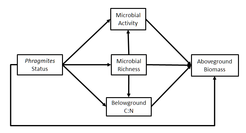
In this case, the variable “Phragmites status” corresponds to the three community types and can’t be represented using a single coefficient. Thus, the marginal-means approach is ideal to elucidate the effect of each community type on both proximate and ultimate ecosystem properties while testing the overall significance of this path.
Let’s read in the data and construct the model:
bowen <- read.csv("https://raw.githubusercontent.com/jslefche/sem_book/master/data/bowen.csv")

bowen <- na.omit(bowen)

library(nlme)

bowen_sem <- psem(
  lme(observed_otus ~ status, random = ~1|Genotype, data = bowen, method = "ML"),
  lme(RNA.DNA ~ status + observed_otus, random = ~1|Genotype, data = bowen, method = "ML"),
  lme(below.C ~ observed_otus + status, random = ~1|Genotype, data = bowen, method = "ML"),
  lme(abovebiomass_g ~ RNA.DNA + observed_otus + belowCN + status, random = ~1|Genotype, data = bowen, method = "ML"),
  data = bowen
)
And let’s retrieve the output:
summary(bowen_sem, .progressBar = FALSE)## Warning: Categorical or non-linear variables detected. Please refer to
## documentation for interpretation of Estimates!##
## Structural Equation Model of bowen_sem
##
## Call:
## observed_otus ~ status
## RNA.DNA ~ status + observed_otus
## below.C ~ observed_otus + status
## abovebiomass_g ~ RNA.DNA + observed_otus + belowCN + status
##
## AIC
## 1110.030
##
## ---
## Tests of directed separation:
##
## Independ.Claim Test.Type DF Crit.Value P.Value
## observed_otus ~ belowCN + ... coef 57 1.4405 0.1552
## RNA.DNA ~ belowCN + ... coef 56 1.3740 0.1749
## below.C ~ belowCN + ... coef 56 2.7225 0.0086 **
## below.C ~ RNA.DNA + ... coef 56 -0.1762 0.8607
## abovebiomass_g ~ below.C + ... coef 54 -0.4540 0.6516
##
## --
## Global goodness-of-fit:
##
## Chi-Squared = 11.484 with P-value = 0.043 and on 5 degrees of freedom
## Fisher's C = 17.877 with P-value = 0.057 and on 10 degrees of freedom
##
## ---
## Coefficients:
##
## Response Predictor Estimate Std.Error DF Crit.Value P.Value
## observed_otus status - - 2 5.9589 0.0508
## observed_otus status = native 2258.6564 105.8178 12 21.3448 0.0000
## observed_otus status = introduced 2535.07 131.2216 14 19.3190 0.0000
## observed_otus status = invasive 2541.4984 56.6887 12 44.8326 0.0000
## RNA.DNA observed_otus 0 0 57 2.1583 0.0351
## RNA.DNA status - - 2 9.3480 0.0093
## RNA.DNA status = invasive 0.7112 0.0118 12 60.4511 0.0000
## RNA.DNA status = introduced 0.7305 0.0264 14 27.6880 0.0000
## RNA.DNA status = native 0.7844 0.0216 12 36.2988 0.0000
## below.C observed_otus 9e-04 3e-04 57 2.6546 0.0103
## below.C status - - 2 17.1995 0.0002
## below.C status = introduced 42.6366 0.3673 14 116.0774 0.0000
## below.C status = invasive 43.4004 0.1594 12 272.2299 0.0000
## below.C status = native 44.4975 0.3056 12 145.6071 0.0000
## abovebiomass_g RNA.DNA -1.8517 1.8893 55 -0.9801 0.3313
## abovebiomass_g observed_otus -2e-04 2e-04 55 -0.7521 0.4552
## abovebiomass_g belowCN 0.005 0.0041 55 1.2026 0.2343
## abovebiomass_g status - - 2 12.9519 0.0015
## abovebiomass_g status = native 1.7489 0.2206 12 7.9272 0.0000
## abovebiomass_g status = invasive 1.8807 0.1041 12 18.0629 0.0000
## abovebiomass_g status = introduced 2.7024 0.232 14 11.6457 0.0000
## Std.Estimate
## -
## - ***
## - ***
## - ***
## 0.135 *
## - **
## - ***
## - ***
## - ***
## 0.2913 *
## - ***
## - ***
## - ***
## - ***
## -0.1428
## -0.0905
## 0.1356
## - **
## - ***
## - ***
## - ***
##
## Signif. codes: 0 '***' 0.001 '**' 0.01 '*' 0.05
##
## ---
## Individual R-squared:
##
## Response method Marginal Conditional
## observed_otus none 0.10 0.19
## RNA.DNA none 0.31 0.81
## below.C none 0.26 0.32
## abovebiomass_g none 0.22 0.28In this case, it appears that the model fits the data well enough based on the Fisher’s C statistic (P = 0.057), which is what the original authors used. Note that the likelihood-based \(\chi^2\) statistic actually implies poor fit (P = 0.043). In this case, examining the d-sep tests suggests the inclusion of the path from \(belowCN\) to \(below.C\) might improve the fit. However, we are applying a tool that was not available to the original authors, so we will proceed as they did and assume adequate fit.
The linkage between microbial community type (\(status\)) and richness (\(observed_otus\)) is non-significant, but the other paths are significant. Examination of the marginal means indicates microbial activity (\(RNA.DNA\)) and belowground carbon (\(below.C\)) are generally highest in Phragmites with native microbial communities based on the post-hoc tests. However, none of these properties appear to influence the ultimate production of biomass (\(abovebiomass_g\)). Rather, that property appears to be entirely controlled by the plant microbiome type (\(status\)): those with the introduced microbial community have significantly higher aboveground biomass based on their marginal mean after controlling for microbial activity and soil nutrients.
Thus, despite a multi-level categorical predictor (\(status\)), the two-step procedure of ANOVA and calculation of marginal means allows for a more mechanistic understanding of the drivers of plant biomass in this species.
5.4 Endogenous Categorical Variables
Endogenous categorical variables are far trickier, and at the moment, are not implemented in piecewiseSEM.
In the case of endogenous categorical variables in a piecewise framework, there are really only two solutions:
for binary variables, set the values as 0 or 1 and model as numeric, which would yield a single coefficient.
for ordinal variables, set the values depending on the order of the factor, e.g., small = 1 < medium = 2 < large = 3, and then model as numeric, which would yield a single coefficient.
Nominal variables (i.e., levels are not ordered) could be modeled using multinomial regression, although this method would have to be executed by hand. An alternative is to use the factor levels to construct a composite variable, the subject of a later chapter. lavaan provides a robust alternative in the form of confirmatory factor analysis (see http://lavaan.ugent.be/tutorial/cat.html). In piecewiseSEM, composites must be constructed by hand, although this procedure is not hugely prohibitive.
5.5 References
Bowen, J. L., Kearns, P. J., Byrnes, J. E., Wigginton, S., Allen, W. J., Greenwood, M., … & Meyerson, L. A. (2017). Lineage overwhelms environmental conditions in determining rhizosphere bacterial community structure in a cosmopolitan invasive plant. Nature communications, 8(1), 433.