3 Local Estimation
3.1 Global vs. local estimation
In the previous chapter, we explored the use of structural equation modeling to estimate relationships among a network of variables based on attempts to reproduce a single variance-covariance matrix. We refer to this approach as global estimation because the variance-covariance matrix captures relationships among all variables in the model at once.
This previous approach comes with a number of assumptions about the data, notably that they are multivariate normal and sufficiently replicated to generate unbiased parameter estimates. However, most data–particularly ecological data–violate these assumptions. Given the difficulty with which the data are collected and the complexity of the proposed relationships, issues with power are often encountered.
While variance-covariance based methods have been extended to consider special cases such as non-normality, an alternative estimation procedure was proposed in 2000 by Shipley based on concepts from graph theory. In this method, relationships for each endogenous (response) variable are estimated separately, which is why we call it local estimation or piecewise SEM, due to the nature by which the model is pieced together.
Recall that global estimation assumes linear relationships, and indeed we have seen in the previous chapter that fitting a SEM and comparing the output with that from a linear model can yield the same results. Local estimation takes the latter approach: fitting a linear model for each response and then stringing together the inferences, rather than trying to estimate all relationships at once. Thus, piecewise SEM is more like putting together a puzzle piece by piece, rather than painting the image on a single canvas.
This approach imparts great flexibility because the assumptions pertaining to each response can be evaluated and addressed individually rather than treating every variable as arising from the same data-generating process.
For example, generalized linear models can be fit for data that are non-Gaussian such as count (e.g., abundance), proportion (e.g., survival), or binary outcomes (e.g., presence-absence). Mixed-effects or hierarchical models can be fit for data that are nested or adhere to some predefined structure. Similarly, non-independence (such as spatial, temporal, or phylogenetic) can be incorporated into the model structure to provide more robust parameter estimates. Moreover, only enough data is needed to be able to fit and estimate each individual regression. In doing so, Shipley’s method relaxes many of the assumptions associated with global estimation and better reflects the types and quantity of data collected by modern ecologists.
A key point to be made is that the piecewise approach does not absolve the user of all assumptions associated with the statistical tests. The data must still meet the assumption of the individual models: for example, most linear regression assume constant variance and independence of errors. Such assumptions still hold, but they can be easily evaluated using the suite of tools already available for said models (e.g., histograms of residuals plots, Q-Q plots, etc.).
However, recall that the goodness-of-fit measures for variance-covariance based structural equation models derive from comparison of the observed vs. estimated variance-covariance matrix. Because local estimation produces a separate variance-covariance matrix for each modeled response, there is no immediate extension from global methods. Instead, Shipley proposed a new test based on directed acyclic graphs (or DAGs).
DAGs are the pictorial representation of the hypothesized causal relationships: in other words, the path diagram. It’s important to point out quickly that DAGs assume recursive relationships, or the absence of feedback loops or bidirectional relationships. Thus, local estimation is unsuitable for such approaches and one must resort to a global approach (with some additional conditions for such model structures).
There is a rich literature pertaining to DAGs, principally in their estimation and evaluation, and Shipley has drawn on this to propose a new index of model fit.
More recently, Shipley and Douma have introduced a more flexible method based on log-likelihood that produces a \(\chi^2\) statistic whose interpretation is much closer to that of global estimation, but further relaxes assumptions by allowing for model assessment and comparison for any models fit using maximum likelihood estimation.
3.2 Tests of directed separation
In global estimation, comparison of the observed vs. estimated variance-covariance matrix through the \(\chi^2\) statistic asks whether the model-implied relationships deviate substantially from the relationships present in the data. If not, then the model is assumed to fit well, and we can go on to use it for inference.
Another way of thinking about model fit is to ask: are we missing any important paths? Recall that structural equation modeling requires careful specification of a hypothesized structure. In the case of underidentified models (those where there are fewer pieces of known information than parameters to be estimated), this means there are missing relationships that could be present but were not included. Paths might be excluded because there is no a priori reason or mechanism to suspect a causal relationship. Recall that modification indices can be used to test the change in the \(\chi^2\) statistic (i.e., how well the model fits) with the inclusion of these missing paths.
The tests of directed separation evaluate this hypothesis more directly by actually fitting the missing relationships to test whether the path coefficients are significantly different from zero, and there whether we are justified in excluding them. This question is actually implicit in the \(\chi^2\) statistic: a substantial deviation from the observed correlations suggests that we’re missing information in our model that could bring our estimates more in line with our observations.
Two variables are said to be d-separated if they are statistically independent conditional on their joint influences. Let’s unpack this statement:
First, the “two variables” are unrelated in the hypothesized causal model: in other words, there is not a directed path already connecting them. Second, we test for “statistical dependence” in our model all the time: the P-values associated with the path coefficients, for example, test whether the effect is significantly different than zero. Statistical independence then asks whether the two variables are significantly unrelated, or that that their relationship is in fact no different from zero. Finally, “conditional on their joint influences” means that the test for statistical independence must account for contributions from already specified influences. In other words, the test must consider the partial effect of one variable on the other if either or both are already connected to other variables in the model.
Procedurally, this evaluation is quite easy: identify the sets of missing relationships, test whether the effect is not significantly different from zero (P > 0.05) controlling for covariates already specified in the model, and combine those inferences to gauge the overall trustworthiness of the model.
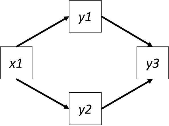
Let’s consider a simple path diagram:
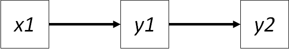
In this case, we have specified two sets of directed relationships: \(x1 -> y1\) and \(y1 -> y2\).
If we apply the t-rule from the chapter on global estimation, we have \(3(3+1)/2\) or 6 pieces of known information (the variances on the 3 variables + the 3 sets of covariances). We want to estimate the 2 parameters \(\gamma_{x1y1}\) and \(\beta_{y1y2}\) and the variances on the 3 variables (we can get their covariances from that). Thus we have 6 known values to estimate 5 unknown values, and the model is overidentified. We noted in the chapter on global estimation that the number of leftover known values can be used as degrees of freedom in the \(\chi^2\) goodness-of-fit test. In this case, there is 1 degree of freedom, so likewise, we can go on to test model fit.
This 1 degree of freedom actually corresponds to the missing relationship between \(x1 -> y2\). This is the independence claim we wish to test: that there is in fact no relationship between \(x1\) and \(y2\). However, the effect of \(x1\) on \(y2\) must be independent (or the partial effect) of the known influence of \(y1\). Thus, we are testing the partial effect of \(x1\) on \(y2\) given \(y1\). You may see this claim written in the following notation: \(x1 | y2 (y1)\) where the bar separates the two variables in the claim, and any conditioning variables follow in parantheses. (Shipley actually puts the two variables in parentheses followed by the conditioning variables in brackets: \((x1, y2) | {y1}\), for the record.)
In this simple example, there is one conditioning variable for the single independence claim. This one independence claim constitutes what is called the basis set, which is the minimum number of independence claims derived from a path diagram. The key word to take away here is minimum.
We could have just as easily tested the claim \(y2 | x1 (y1)\), which is the same relationship but in the opposite direction. However, the statistical test or P-value associated with this relationship is the same regardless of the direction. In other words, the partial effect of \(x1\) on \(y2\) is the same as \(y2\) on \(x1\) (although there is a caveat to this claim for GLM, which we will address later). In such a case, we would include only the one claim rather than both claims that provide the same information.
Therefore, our first rule of directed separation is: the sum number of independence claims in the basis set cannot be derived from some combination of the others within it.
As an aside, if we add this claim back into the model, we would have no missing paths. Thus, no independence claims or tests of directed separation would be possible. As is the case with \(\chi^2\), we would not have any leftover information with which to test model fit. This does not preclude fitting the model and drawing inference, only that its goodness-of-fit cannot be assessed. However, there are other qualitative ways of assessing model fit, such as looking that proportion of variance or deviance explained for each endogenous variable (i.e., \(R^2\)) and assessing the significance of the individual paths. If a high proportion of variance is explained in all endogenous variable and there are significant path coefficients, it follows that residual error is low, and it’s safe to assume that there are no other variables out there that can further clarify the model structure. Nevertheless, you should be open about why you chose to fit a just identified model, and why you are not reporting any goodness-of-fit statitsics.
As path diagrams become more complex, the natural question is: how far back do you go in terms of conditioning? Take the following example:
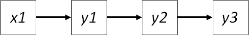
There are several missing paths: \(x1 -> y2\), \(x1 -> y3\) and \(y1 -> y3\).
Let’s consider the independence claim \(x1 -> y3\). Based on our last example, \(y2\) must be included as a conditioning variable due to its direct influence on \(y3\), but what about \(y1\)? It has an indirect influence on \(y3\) through \(y2\). However, by having included \(y2\) in the independence claim, we have already (theoretically) incorporated the indirect influence of \(y1\) in the form of variation in \(y2\). In other words, any effect of \(y1\) would change \(y2\) before \(y3\), and the variance in \(y2\) is already considered in the independence claim. So the full claim would be simply: \(x1 | y3 (y2)\).
Our second rule of the d-sep test is: conditioning variables consist of only those variables immediate to the two variables whose independence is being evaluated.
In other words, we assume that the effects of any other downstream variables are captured in the variance contributed by the immediate ancestors, and we can therefore ignore them. Upstream variables (those occurring later in the path diagram beyond both variables included in the claim) are never considered as conditioning variables, for the obvious reason that causes cannot precede effects.
For the claim \(y1 -> y3\) above, there are now two conditioning variables: \(y2\) (on \(y3\)) and also \(x1\) (on \(y1\)). So the final independence claim would be: \(y1 | y3 (x1, y1)\). Note that the effect of \(y1\) on \(y2\) is not included, because it is too ancestral.
The full basis set for this diagram would then be:
- \(x1 | y3 (y2)\)
- \(y1 | y3 (y2, x1)\)
- \(x1 | y2 (y1)\)
Deriving the basis set can be difficult but mercifully is automated in the piecewiseSEM package. This package makes some choices about the basis set that deviate from the recommendations of Shipley. For example, consider the following path diagram:
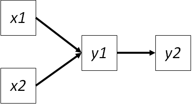
The basis set includes the unspecified paths from \(x1 | y2 (y1)\) and \(x2 | y2 (y1)\). But what about \(x1 | x2\)?
Shipley would include this claim in the basis set. However, several argument could be made against it along several fronts.
First, unlike \(y2\) which very clearly is an effect (i.e., has a directed path flowing into it), there is no expectation of a cause-effect relationship between the two exogenous variables \(x1\) and \(x2\). In fact, such a relationship may yield nonsensical claims (e.g., between study area and month) or claims where directionality is confounded in one direction (e.g., latitude drives variation in species richness, but species richness does not change the latitude of the Earth). If the purpose of the test is to evaluate linkages that were originally deemed irrelevant, is it really that useful to test non-mechanistic or impossible links? If we did indeed recover a significant correlation between study area and month, is that mechanistically meaningful? Why should the area over which the study was conducted change due to the time of the study? And should we therefore reject a model due to a totally spurious relationship? These are tough questions with no clear answer. From a personal perspective, I believe the tests of directed separation should be diagnostic: should I have included this path? Did it provide useful information? Including non-informative claims because they can be evaluated simply inflates type II error (i.e., you are more likely to falsely accept the model) with no real benefit to the identifying underlying causal processes.
Second, and more practically, there is no easy way for the user to specify the distributional and other assumptions associated with exogenous variables in the same way they can for endogenous variables. By virtue of modeling \(y2\) in a directed path (from \(y1\)), the user has made it clear in the coding of the model how that response should be treated. However, no where in the regression models is there information on how \(x1\) should be treated: is it binomial? Hierarchical? Polynomial? Asking the user to code this information would vastly inflate the amount of code necessary to run tests, and combined with the above, would yield little insight for a potentially very large hindrance.
Nevertheless, independence claims could be added back into the basis set if the user decides they disagree with this perspective.
Now that we are comfortable identifying missing paths and constructing the basis set, the next step is to test them for statistical independence. This can be done by taking the response as it is treated in the original model, and swapping the predictors with those in the independence claim. The way, the assumptions of the endogenous variable are preserved. So, for example, if \(y3\) in the previous path model is binomally-distributed as a function of \(y2\), then any independence claims involving \(y2\) would also treat is as binomial.
Once the model is fit, statistical independence is assessed with a t-, F-, or other test. If the resulting P-value is >0.05, then we fail to reject the null hypothesis that the two variables are conditionally independent. In this case, a high P-value is a good thing: it indicates that we were justified in excluding that relationship from our path diagram in the first place, because the data don’t support a strong linkage between those variables within some tolerance for error.
Shipley’s most important contribution was to show that the P-values can be summed to construct a fit index analogous to the \(\chi^2\) statistic from global estimation: Fisher’s C statistic, which is calculated as:
\[C = -2{\sum_{i=1}^k ln(p_i)}\]
where \(k\) is the number of independence claims in the basis set, i is the ith claim, and p is the P-value from the corresponding significance test.
Furthermore, Shipley showed that C is \(\chi^2\) distributed with 2\(k\) degrees of freedom. Thus, a model-wide P-value can be obtained by comparing the value to a \(\chi^2\) table with the appropriate degrees of freedom.
As with the \(\chi^2\) test in global estimation, a model-wide P > 0.05 is desirable because it implies that the hypothesized structure is supported by the data. In other words, no potentially significant missing paths were excluded.
Like the \(\chi^2\) difference test, the C statistic can be used to compare nested models. Shipley later showed that the the C statistic can also be used to compute an AIC score for the SEM:
\[AIC = C + 2K\]
where \(K\) is the likelihood degrees of freedom (not \(k\), the number of claims in the basis set). A further variant for small sample sizes, \(AIC_c\), can be obtained by adding an additional penalty:
\[AIC_c = C + 2K\frac{n}{(n - K - 1)}\]
It’s important to point out that, like the \(\chi^2\) statistic for global estimation, the C statistic can be affected by sample size, but not in as direct a way. As sample size increases, the probability of recovering a “significant” P-vaue increases, reducing the potential for a good-fitting model. Similarly, more complex models may lead to a kind of “overfitting” where significant d-sep tests are obscured by many more non-significant values leading to strong support for the (potentially incorrect) model structure. Paradoxically, poor sample size can also lead to a good-fitting model because the tests lack the power to detect an actual effect (high Type II error), leading to the paradoxical situation of a well-supported model whose paths are all non-significant. Such biases should be considered when reporting the results of the test, and the tolerance of error (i.e., \(\alpha\)) could be adjusted for larger datasets.
In this way, the tests of directed separation may be usefully diagnostic by drawing attention to the specific relationships that could be re-inserted into the model, which would have the added benefit of improving model fit by removing those significant P-values from the basis set. Whether this is advisable depends on the goal of the exercise: in an “exploratory” mode, for example, adding paths might be useful if they are theoretically justifiable. I would not, however, recommend selecting all non-significant paths and reinserting them into the model to improve model fit, or iteratively re-adding paths until adequate fit is achieved. Keep in mind that those paths were not included in the original path diagram because you, the user, did not consider them important. Why would you put them back into the model? Rather, perhaps it is the original model structure or the data that is inadequate, and you should consider alternative formulations, additional covariates, or other modifications to better reflect the reality suggested by the data.
3.3 A Log-Likelihood Approach to Assessing Model Fit
Recently, Shipley and Douma developed an alternative index of model fit using maximum likelihood. You will recall from the chapter on global estimation that maximum likelihood estimation searches over parameter space for the values of the coefficients \(\theta\) that maximize the probability \(P\) of having observed your data \(X\). The likelihood \(L\) of the model is therefore the value produced by this function when \(P\) is maximized by the model-estimated coefficients \(\hat{\theta}\): \(L(\hat{\theta} | X)\).
This is often reported as the log-likelihood (the log of this value) as it simplifies the calculation of the fitting function for common statistical distributions: \(log(L(\hat{\theta} | X))\).
Each component model in the SEM produces a log-likelihood, assuming it is fit using maximum likelihood estimation. The log-likelihood of the full set of structural equations \(M\) is therefore the sum of the individual log-likelihood values for each of the submodels (based on Markov decomposition of the joint probability distribution):
\[log(L_M(\theta | X)) = {\sum_{i=1}^k log(L_i(\theta_i | X_i)}\]
This global quantity summarizes the likelihood associated with ALL of the coefficients across all models.
Recall from the global estimation chapter that the objective there is to minimize the discrepancy between the model estimated and observed variance-covariance matrices. This is essentially testing whether the covariance between unlinked variables is zero. Take this model from that chapter:
Here, the assumption is that the covariance between \(x1\) and \(y2\) is zero. In other words, by omitting a direct path between them, we are claiming that they are conditionally independent or causally unrelated. Deviations from this assumption will cause the model-estimated variance-covariance matrix to pull away from from the observed matrix, causing the \(F_{ML}\) to increase, the likelihood to decline, and the fit to become increasingly poor.
In a piecewise context, we could rewrite the structural equation \(y2 ~ y1\) to be \(y2 ~ y1 + 0*x1\) to reflect our assumption that the coefficient for the relationship between \(x1\) and \(y2\) is zero. This is different from the equation \(y2 ~ y1 + x1\), which would produce an estimate for this relationship. In the d-sep tests, we actually fit this second model and extract the P-value associated with this estimate. If P>0.05, we validate our original assumption that the two are independent, conditional on \(y1\). But it could just as easily not be zero, and we would reject the fit of the model.
We can also produce a log-likelihood for this second model that allows \(x1\) to vary freely. A likelihood ratio test would then allow us to tell whether the second model was more or less likely within some tolerance for error. If the second model is more likely, they we were incorrect in assuming the relationship between \(x1\) and \(y2\) is zero, and our original formulation could be considered a poor representation of the data.
Shipley and Douma showed that this procedure can be extended to the entire SEM, first by incorporating ALL missing paths (or the variables whose covariances we assume to be 0), then taking the difference in log-likelihoods for each submodel between the proposed model and the one with all paths accounted for, and finally summarizing these differences to get an overall index of model fit.
How, then, to re-fit the models including the missing parameters? We already have a handy blueprint in the form of the basis set, which tells us which relationships are missing. We can reparameterize the models to include the missing paths specified in the basis set, extract the log-likelihood, and compare that value to the log-likelihood of the original models. Because this procedure would require all variables to be linked, this procedure is essentially fitting a fully saturated model (i.e., all variables are linked) and comparing it to a nested model where some paths are missing. Note that this test is not possible for models that are already saturated, which is also true for global estimation.
If we assume the fully saturated model \(M_2\) and the proposed (nested) model \(M_1\), Shipley and Douma show that the \(\chi^2\) statistic can be computed as follows:
\[\chi^2_ML = -2(log(L(M_1)) - log(L(M_2))\] Which can be compared to a \(\chi^2\) distribution with \(k\) degrees of freedom, where \(k\) is the sum of the differences in the likelihood degrees of freedom (number of likelihood-estimated parameters) between each of the submodels in \(M1\) and \(M2\). If we allow the previously unestimated paths to freely vary, but this in turn does not improve the likelihood of the model, then this {^2} value becomes increasingly smaller. In this way, the procedure is the exact analogue of the classic \(F_{ML}\) in global estimation, we also seeks to minimize these differences between two matrices. As we shall see, they actually produce identical results when we assume normality.
As AIC is simply the log-likelihood penalized for complexity, Shipley and Douma go on to show that a model-wide AIC value can be derived as the sum of the AIC values for each submodel i in \(M1\):
\[AIC_{M1} = {\sum_{i=1}^v AIC_i}\] Note that this is not the difference in AIC values between the proposed and saturated models. Additionally, a corrected \(AIC_c\) can be substituted for small sample sizes.
Note that the AIC obtained from the d-sep tests cannot be compared with that derived from likelihood, and vice versa.
What is useful about this method is that it brings the technique more in parity with variance-covariance based SEM, and solves several outstanding issues associated with the d-sep tests, namely:
- d-sep tests consider only changes in topology so it is only useful when comparing models that differ in their independence claims, whereas a log-likelihood approach considers all changes to the model above and beyond the DAG, such as changing the underlying distribution (which changes the maximum likelihood fitting function) or random effects.
- this method can be applied for all models fit using maximum likelihood, including truly non-linear approaches such as generalized additive models (GAMs). Note, however, that GAMs do not produce traditional linear coefficients (but rather fitted smoothing functions), so there are still downsides with respect to paramterizing the DAG and drawing inference.
- it omits issues associated with reporting P-values for mixed models where the denominator degrees of freedom are unclear (see: lme4).
This method cannot be used when the conditions for maximum likelihood are not met, such as for regresson on distance matrices, and so in these cases, only test of directed separation are possible. Nevertheless, log-likelihood based {^2} is an incredibly useful addition and will likely become the default goodness-of-fit metric moving forward due to its flexibility and similarity to traditional methods.
3.4 Model fitting using piecewiseSEM
Fitting a piecewise structural equation model is as simple as fitting each regression separately: if you can fit an lm in R, you have already fit a SEM!
The package of course is piecewiseSEM:
library(piecewiseSEM)And let’s return to the data from Grace & Keeley (2006) that we explored in the chapter on global estimation:
data(keeley)As a reminder, Grace & Keeley wanted to understand patterns in plant diversity following disturbance, in this case wildfires in California.
In the end of the global estimation chapter, we tested for full mediation using the following model:
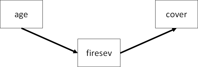
As in lavaan, it’s first necessary to break down the list of structural equations. Unlike lavaan these are not coded as character strings, but instead as full-fledged linear models. You can see where coding each model separately will impart greater flexibility, for example, by fitting a GLM, mixed-effects model, and so on.
Rather than using the function sem, the list of models are put together using the function psem which is the primary workhouse of the piecewiseSEM package.
keeley_psem <- psem(
  lm(cover ~ firesev, data = keeley),
  lm(firesev ~ age, data = keeley),
  data = keeley)
Note: It’s not necessary to pass a data argument to psem but it can help alleviate errors in certain cases.
Before we get to the model fitting, let’s just examine the psem object by itself:
keeley_psem## Structural Equations of x :
## lm: cover ~ firesev
## lm: firesev ~ age
##
## Data:
## distance elev abiotic age hetero firesev cover rich
## 1 53.40900 1225 60.67103 40 0.757065 3.50 1.0387974 51
## 2 37.03745 60 40.94291 25 0.491340 4.05 0.4775924 31
## 3 53.69565 200 50.98805 15 0.844485 2.60 0.9489357 71
## 4 53.69565 200 61.15633 15 0.690847 2.90 1.1949002 64
## 5 51.95985 970 46.66807 23 0.545628 4.30 1.2981890 68
## 6 51.95985 970 39.82357 24 0.652895 4.00 1.1734866 34
## ...with 84 more rows
##
## [1] "class(psem)"It returns the submodels, their classes (in this case lm), and a snippet of the data.
The first step is to derive the basis set using the function basisSet:
basisSet(keeley_psem)## $`1`
## [1] "age | cover ( firesev )"Here, there is a single independence claim representing the missing path from \(age -> cover\) conditional on the influence of \(firesev\) on \(cover\).
Now to evaluate the tests of directed separation using the function dSep:
dSep(keeley_psem, .progressBar = FALSE)## Independ.Claim Test.Type DF Crit.Value P.Value
## 1 cover ~ age + ... coef 87 -1.80184 0.07503437Note that the output is the same as if we evaluated the independence claim ourselves:
summary(lm(cover ~ firesev + age, data = keeley))$coefficients[3, ]## Estimate Std. Error t value Pr(>|t|)
## -0.004832969 0.002682241 -1.801839905 0.075034374Now, we can compute the Fisher’s C statistic using the P-value obtained from the d-sep test. Recall that the degrees of freedom for the test is twice the number of independence claims, so in this case \(2*1 = 2\). We can use these values to compare the statistic to a \(\chi^2\) distribution to get a model-wide P-value:
(C <- -2 * log(summary(lm(cover ~ firesev + age, data = keeley))$coefficients[3, 4]))## [1] 5.1796181-pchisq(C, 2)## [1] 0.07503437So in this case, we would fail to reject the model as P>0.05. Note that in the case of a single independence claim, the model-wide P-value is the same as the P-value for the individual claim.
Alternatively, we could just use the function fisherC which constructs the statistic for us:
fisherC(keeley_psem)## Fisher.C df P.Value
## 1 5.18 2 0.075Let’s now compute the log-likelihood based \(\chi^2\) statistic to see if we get the same answer. To do so, we must first create the saturated model, which in this case would involve fitting a path between \(age\) and \(cover\):
keeley_psem2 <- psem(
  lm(cover ~ firesev + age, data = keeley),
  lm(firesev ~ age, data = keeley),
  data = keeley
)
From here, we can get the log-likelihoods of both submodels using the logLik function for each SEM, take their difference, and construct the \(\chi^2\) statistic:
LL_1 <- logLik(lm(cover ~ firesev, data = keeley)) - logLik(lm(cover ~ firesev + age, data = keeley))

LL_2 <- logLik(lm(firesev ~ age, data = keeley)) - logLik(lm(firesev ~ age, data = keeley))

(ChiSq <- -2*sum(as.numeric(LL_1), as.numeric(LL_2)))
## [1] 3.297429DF <- 1 # one additional parameter estimated in the saturated model
1 - pchisq(ChiSq, DF)## [1] 0.06938839So we would also fail to reject the model based on the P-value obtained from this test. We can more easily obtain the same output using the function LLchisq on the original (unsaturated) model:
LLchisq(keeley_psem)## Chisq df P.Value
## 1 3.297 1 0.069Note for models assuming multivariate normality (as we have here), the {^2} statistic and P-value are actually the same as we obtain from lavaan:
library(lavaan)## This is lavaan 0.6-9
## lavaan is FREE software! Please report any bugs.keeley_formula <- '
firesev ~ age
cover ~ firesev
'
keeley_sem <- sem(keeley_formula, data = keeley)
fit <- lavInspect(keeley_sem, "fit")
fit["chisq"]; fit["pvalue"]## chisq
## 3.297429## pvalue
## 0.06938839Note that we can also obtain an AIC score for the model. The default is based on the log-likelihood \(\chi^2\) and we shall see why in a minute:
AIC(keeley_psem)## AIC K n
## 1 364.696 6 90To get the AIC value based on the Fisher’s C statistic and the d-sep tests, we can add the following argument:
AIC(keeley_psem, AIC.type = "dsep")## AIC K n
## 1 17.18 6 90Ah, a fully saturated or just identified model will yield a C statistic of 0. Based on Shipley’s equation above, the AIC score reduces to \(2K\), or twice the likelihood degrees of freedom. This is in contrast to alternative formulation, which is based on actual likelihoods. Therefore, in situations where one wishes to compare a model that is fully saturated, we advise using the default \(\chi^2\)-based value.
This exercise was a long workaround to reveal that all the above can be executed simultaneously using the summary function on the SEM object:
summary(keeley_psem, .progressBar = FALSE)##
## Structural Equation Model of keeley_psem
##
## Call:
## cover ~ firesev
## firesev ~ age
##
## AIC
## 364.696
##
## ---
## Tests of directed separation:
##
## Independ.Claim Test.Type DF Crit.Value P.Value
## cover ~ age + ... coef 87 -1.8018 0.075
##
## --
## Global goodness-of-fit:
##
## Chi-Squared = 3.297 with P-value = 0.069 and on 1 degrees of freedom
## Fisher's C = 5.18 with P-value = 0.075 and on 2 degrees of freedom
##
## ---
## Coefficients:
##
## Response Predictor Estimate Std.Error DF Crit.Value P.Value Std.Estimate
## cover firesev -0.0839 0.0184 88 -4.5594 0 -0.4371 ***
## firesev age 0.0597 0.0125 88 4.7781 0 0.4539 ***
##
## Signif. codes: 0 '***' 0.001 '**' 0.01 '*' 0.05
##
## ---
## Individual R-squared:
##
## Response method R.squared
## cover none 0.19
## firesev none 0.21The output should look very familar to the output from other summary calls, like summary.lm. The d-sep tests, \(\chi^2\) and Fisher’s C tests of goodness-of-fit, and AIC are all reported.
Additionally, model coefficients are returned. Unlike lavaan, the standardized estimates are provided by default. Also unlike lavaan, the individual model \(R^2\) values are also returned by default. Both sets of statistics are key for inference, and thus we have decided to make them available with any further arguments passed to summary.
We can compare the piecewiseSEM output to the lavaan output:
library(lavaan)

sem1 <- '
firesev ~ age
cover ~ firesev
'

keeley_sem1 <- sem(sem1, keeley)

summary(keeley_sem1, standardize = T, rsq = T)
## lavaan 0.6-9 ended normally after 19 iterations
##
## Estimator ML
## Optimization method NLMINB
## Number of model parameters 4
##
## Number of observations 90
##
## Model Test User Model:
##
## Test statistic 3.297
## Degrees of freedom 1
## P-value (Chi-square) 0.069
##
## Parameter Estimates:
##
## Standard errors Standard
## Information Expected
## Information saturated (h1) model Structured
##
## Regressions:
## Estimate Std.Err z-value P(>|z|) Std.lv Std.all
## firesev ~
## age 0.060 0.012 4.832 0.000 0.060 0.454
## cover ~
## firesev -0.084 0.018 -4.611 0.000 -0.084 -0.437
##
## Variances:
## Estimate Std.Err z-value P(>|z|) Std.lv Std.all
## .firesev 2.144 0.320 6.708 0.000 2.144 0.794
## .cover 0.081 0.012 6.708 0.000 0.081 0.809
##
## R-Square:
## Estimate
## firesev 0.206
## cover 0.191Again, because we are making the same assumptions as for global estimation (i.e., multivariate normality), all of the output will be identical (or nearly identical based on rounding and optimization differences).
Of course, we might expect greater divergence between the two methods if we were to incorporate different distributions and more complex model structures, which we will explore now.
3.5 Extensions to Generalized Mixed Effects Models
Let’s turn to the example from Shipley (2009) on tree survival. In this (hypothetical) study, individual trees are followed for 36 years at 20 sites and measured for date of bud burst (Date), cumulative degree days until first bud burst (DD), growth, and survival.
It’s important to note that these data have multiple levels of hierarchical structure: between sites, between individuals within sites, between years within individuals within sites. They also have non-normal responses: survival is measured as a binary outcome (alive or dead).
Shipley hypothesized these variables are related in the following way:

Let’s first treat the data as normal and independent using lavaan:
data(shipley)

shipley_model <- '
DD ~ lat
Date ~ DD
Growth ~ Date
Live ~ Growth
'

shipley_sem <- sem(shipley_model, shipley)

summary(shipley_sem, standardize = T, rsq = T)
## lavaan 0.6-9 ended normally after 27 iterations
##
## Estimator ML
## Optimization method NLMINB
## Number of model parameters 8
##
## Used Total
## Number of observations 1431 1900
##
## Model Test User Model:
##
## Test statistic 38.433
## Degrees of freedom 6
## P-value (Chi-square) 0.000
##
## Parameter Estimates:
##
## Standard errors Standard
## Information Expected
## Information saturated (h1) model Structured
##
## Regressions:
## Estimate Std.Err z-value P(>|z|) Std.lv Std.all
## DD ~
## lat -0.860 0.023 -37.923 0.000 -0.860 -0.708
## Date ~
## DD -0.517 0.016 -32.525 0.000 -0.517 -0.652
## Growth ~
## Date 0.173 0.020 8.508 0.000 0.173 0.219
## Live ~
## Growth 0.006 0.001 9.854 0.000 0.006 0.252
##
## Variances:
## Estimate Std.Err z-value P(>|z|) Std.lv Std.all
## .DD 52.628 1.967 26.749 0.000 52.628 0.499
## .Date 38.080 1.424 26.749 0.000 38.080 0.575
## .Growth 38.981 1.457 26.749 0.000 38.981 0.952
## .Live 0.025 0.001 26.749 0.000 0.025 0.936
##
## R-Square:
## Estimate
## DD 0.501
## Date 0.425
## Growth 0.048
## Live 0.064First, we notice the goodness-of-fit can be estimated, but the model is a poor fit (P<0.001). The paths are all significant but this doesn’t do us much good considering the model is not suitable for inference.
Instead of fiddling with modification indices and trying to rejigger the model strcuture, let’s analyze the same path diagram using a piecewise approach and recognizing both the hierarchical structure AND non-normality of the data. For this we will use two common packages for mixed-effects models, lme4 and nlme:
library(nlme)
library(lme4)

shipley_psem <- psem(

  lme(DD ~ lat, random = ~ 1 | site / tree, na.action = na.omit,
  data = shipley),

  lme(Date ~ DD, random = ~ 1 | site / tree, na.action = na.omit,
  data = shipley),

  lme(Growth ~ Date, random = ~ 1 | site / tree, na.action = na.omit,
  data = shipley),

  glmer(Live ~ Growth + (1 | site) + (1 | tree),
  family = binomial(link = "logit"), data = shipley)

  )

summary(shipley_psem, .progressBar = FALSE)
##
## Structural Equation Model of shipley_psem
##
## Call:
## DD ~ lat
## Date ~ DD
## Growth ~ Date
## Live ~ Growth
##
## AIC
## 21745.782
##
## ---
## Tests of directed separation:
##
## Independ.Claim Test.Type DF Crit.Value P.Value
## Date ~ lat + ... coef 18 -0.0798 0.9373
## Growth ~ lat + ... coef 18 -0.8929 0.3837
## Live ~ lat + ... coef 1431 1.0280 0.3039
## Growth ~ DD + ... coef 1329 -0.2967 0.7667
## Live ~ DD + ... coef 1431 1.0046 0.3151
## Live ~ Date + ... coef 1431 -1.5617 0.1184
##
## --
## Global goodness-of-fit:
##
## Chi-Squared = NA with P-value = NA and on 6 degrees of freedom
## Fisher's C = 11.536 with P-value = 0.484 and on 12 degrees of freedom
##
## ---
## Coefficients:
##
## Response Predictor Estimate Std.Error DF Crit.Value P.Value Std.Estimate
## DD lat -0.8355 0.1194 18 -6.9960 0 -0.6877 ***
## Date DD -0.4976 0.0049 1330 -100.8757 0 -0.6281 ***
## Growth Date 0.3007 0.0266 1330 11.2917 0 0.3824 ***
## Live Growth 0.3479 0.0584 1431 5.9552 0 0.7866 ***
##
## Signif. codes: 0 '***' 0.001 '**' 0.01 '*' 0.05
##
## ---
## Individual R-squared:
##
## Response method Marginal Conditional
## DD none 0.49 0.70
## Date none 0.41 0.98
## Growth none 0.11 0.84
## Live delta 0.16 0.18The immediately obvious difference based on Fisher’s C is that the model is no longer a poor fit: we have 12 degrees of freedom corresponding to 6 independence claims, all of which have P > 0.05. Therefore, the model-wide P = 0.484, and we would therefore reject the null that the data do not support the hypothesized model structure.
Moreover, while the direction of the parameter estimates remain the same, they vary considerably in their magnitudes (e.g., \(\beta_{date, DD} = -0.652\) for lavaan and \(\beta_{date, DD} = -0.497\) in piecewiseSEM).
The model \(R^2\)s are all higher as well, for fixed-effects only (marginal) and especially for fixed- and random-effects together (conditional).
Thus, by addressing the non-independence of the data, we have converged on support for the hypothesized model structure, more accurate parameter estimates, and a higher proportion of explained variance than was possible using lavaan.
Note, however, that the model does not report a \(\chi^2\) statistic, and issues a warning about convergence. When one or more of submodels in the saturated SEM fail to converge, it may produce invalid likelihood estimates that lead to the situation where \(\chi^2\)<0. Since this is not permissible, the function returns NA for the \(\chi^2\) statistic and associated P-value. Potential solutions include tweaking model optimizers to ensure a convergent solution, or relying on Fisher’s C.
3.6 Extensions to Non-linear Models
One of the benefits noted above for the newer log-likelihood based goodness-of-fit procedure is that it can be extended to truly non-linear models, such as generalized additive models (GAMs), where maximum likelihood estimation is applied. Let’s now work through an example extending to GAMs.
We’ll work from the random dataset generated in the supplements for the paper by Shipley and Douma. First, let’s generate the data using their code:
set.seed(100)
n <- 100
x1 <- rchisq(n, 7)
mu2 <- 10*x1/(5 + x1)
x2 <- rnorm(n, mu2, 1)
x2[x2 <= 0] <- 0.1
x3 <- rpois(n, lambda = (0.5*x2))
x4 <- rpois(n, lambda = (0.5*x2))
p.x5 <- exp(-0.5*x3 + 0.5*x4)/(1 + exp(-0.5*x3 + 0.5*x4))
x5 <- rbinom(n, size = 1, prob = p.x5)
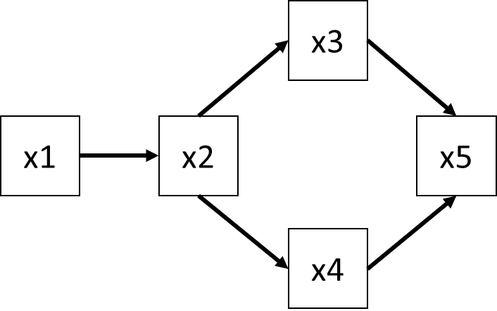
dat2 <- data.frame(x1 = x1, x2 = x2, x3 = x3, x4 = x4, x5 = x5)You’ll note that there is a mix of linear and non-linear variables, including Poisson- and binomial-distributions.
Now let’s consider the SEM from their paper (Figure 1a):
In the paper, Shipley and Douma first fit a strictly linear SEM assuming multivariate normality, which we will also do here:
shipley_psem2 <- psem(
  lm(x2 ~ x1, data = dat2),
  lm(x3 ~ x2, data = dat2),
  lm(x4 ~ x2, data = dat2),
  lm(x5 ~ x3 + x4, data = dat2)
)

LLchisq(shipley_psem2)
## Chisq df P.Value
## 1 4.143 5 0.529We see that, despite having generated data that is inherently non-normal and non-linear, the model is actually a good fit to the data with a P-value of 0.529.
Nevertheless, we know we can do better, both by including non-Gaussian distributions and also through the application of generalized additive models, which model the response not as a linear function of the predictors, but through smoothing functions that allow for non-linear relationships to emerge.
Let’s re-fit the model using a mix of GLMs and GAMs:
library(mgcv)## This is mgcv 1.8-36. For overview type 'help("mgcv-package")'.shipley_psem3 <- psem(
gam(x2 ~ s(x1), data = dat2, family = gaussian),
glm(x3 ~ x2, data = dat2, family = poisson),
gam(x4 ~ x2, data = dat2, family = poisson),
glm(x5 ~ x3 + x4, data = dat2, family = binomial)
)
LLchisq(shipley_psem3)## Chisq df P.Value
## 1 3.346 5 0.647This model also has adequate fit, with a P-value of 0.647. Note that these are the same values reported in Table 2. How to choose among them? Let’s compute the AIC scores (based on log-likelihoods) for both and compare them:
AIC(shipley_psem2, shipley_psem3)## AIC K n
## 1 1240.20 13.000 100
## 2 1190.75 11.563 100We see that the second SEM–the one that better addresses the underlying forms of the data–has much higher support than the straight linear SEM, with the \(\Delta AIC = 49.45\). Thus, we would far and away choose the second model, in line with how Shipley and Douma have designed their simulation.
Now let’s examine the summary output for this second model:
summary(shipley_psem3)## Warning: Categorical or non-linear variables detected. Please refer to
## documentation for interpretation of Estimates!##
## Structural Equation Model of shipley_psem3
##
## Call:
## x2 ~ s(x1)
## x3 ~ x2
## x4 ~ x2
## x5 ~ x3 + x4
##
## AIC
## 1190.750
##
## ---
## Tests of directed separation:
##
## No independence claims present. Tests of directed separation not possible.
##
## --
## Global goodness-of-fit:
##
## Chi-Squared = 3.346 with P-value = 0.647 and on 5 degrees of freedom
## Fisher's C = NA with P-value = NA and on 0 degrees of freedom
##
## ---
## Coefficients:
##
## Response Predictor Estimate Std.Error DF Crit.Value P.Value Std.Estimate
## x2 s(x1) - - 3.2242 41.2590 0e+00 -
## x3 x2 0.1464 0.0373 98.0000 3.9248 1e-04 0.363
## x4 x2 0.1741 0.038 100.0000 4.5856 0e+00 0.3565
## x5 x3 -0.5083 0.1521 97.0000 -3.3414 8e-04 -0.4037
## x5 x4 0.4587 0.1388 97.0000 3.3047 1e-03 0.4414
##
## ***
## ***
## ***
## ***
## ***
##
## Signif. codes: 0 '***' 0.001 '**' 0.01 '*' 0.05
##
## ---
## Individual R-squared:
##
## Response method R.squared
## x2 none 0.57
## x3 nagelkerke 0.21
## x4 none 0.14
## x5 nagelkerke 0.28Most of this should look familiar. Note that the output does not report estimates or standard errors for the smoothed variables. This is because, as noted previously, these are not linear coefficients but instead smoothing functions and there is not a single value relating how, for example, \(x1\) changes with \(x2\). Therefore, calculation of direct and indirect effects is not possible using GAMs, which could make them less than ideal when the goal is to compare the strength of various pathways within a model.
However, it is possible, as we have shown here, to compare among models and validate the topology of the DAG, which in many cases is sufficient to test hypotheses. Those seeking to understand how \(x1\) changes non-linearly with \(x2\) would then have to present additional predicted plots of this relationship in addition to the path diagram.
3.7 A Special Case: Where Graph Theory Fails
In the majority of cases, as we have established, the direction of the independence claim doesn’t matter because, while the coefficients will differ, their P-values will be identical. Thus it doesn’t matter if you test \(y | x\) or \(x | y\) because the claim will yield the same significance test. EXCEPT when intermediate endogenous variables are non-normally distributed.
Consider the following SEM:
In this SEM, there are two independence claims:
- \(y3 | x1 (y1, y2)\)
- \(y2 | y1 (x1)\)
In the second independence claim, if both variables were normally distributed, the significance value is the same whether the test is conducted as \(y2 | y1 (x1)\) or \(y1 | y2 (x1)\). This is NOT true, however, when one or both of the responses are fit to a non-normal distribution. This is because the response is now transformed via a link function \(g(\mu)\) (see chapter on coefficients), and the parameter estimates–and their standard errors–are now expressed on the link scale. This transformation means the P-value obtained by regressing \(y1 ~ y2\) is NOT the same as the one obtained by regressing \(y2 ~ y1\).
To show this is true, let’s generate some Poisson-distributed data and model using both LM and GLM with a log-link:
set.seed(87)

glmdat <- data.frame(x1 = runif(50), y1 = rpois(50, 10), y2 = rpois(50, 50), y3 = runif(50))

# LM
summary(lm(y1 ~ y2 + x1, glmdat))$coefficients[2, 4]
## [1] 0.03377718summary(lm(y2 ~ y1 + x1, glmdat))$coefficients[2, 4]## [1] 0.03377718# GLM
summary(glm(y1 ~ y2 + x1, "poisson", glmdat))$coefficients[2, 4] ## [1] 0.03479666summary(glm(y2 ~ y1 + x1, "poisson", glmdat))$coefficients[2, 4]## [1] 0.08586767In the case of lm the P-value is identical regardless of the direction, and moreover is < 0.05, thus–depending on the outcome of the other claim–we might reject the model.
In contrast, when \(y1\) and \(y2\) are modeled as Poisson-distributed, the P-value is alternatingly < and >= 0.05. Thus, depending on how the claim is specified, we might or might not reject the model. A big difference!
Note that the log-likelihoods are also different for GLM:
logLik(glm(y1 ~ y2 + x1, "poisson", glmdat))## 'log Lik.' -128.8009 (df=3)logLik(glm(y2 ~ y1 + x1, "poisson", glmdat))## 'log Lik.' -158.0841 (df=3)piecewiseSEM solves this by providing three options to the user.
We can specify the directionality of the test if, for instance, it makes greater biological sense to test \(y1\) against \(y2\) instead of the reverse (for example: abundance drives species richness, not vice versa); or
We can remove that path from the basis set and instead specify it as a correlated error using
%~~%. This circumvents the issue altogether but it may not make sense to assume both variables are generated by some underlying process; orWe can conduct both tests and choose the most conservative (i.e., lowest) P-value or maximum difference in the log-likelihoods.
These options are returned by summary in the event the above scenario is identified in the SEM:
glmsem <- psem(
  glm(y1 ~ x1, "poisson", glmdat),
  glm(y2 ~ x1, "poisson", glmdat),
  lm(y3 ~ y1 + y2, glmdat)
)

summary(glmsem)
## Error:
## Non-linearities detected in the basis set where P-values are not symmetrical.
## This can bias the outcome of the tests of directed separation.
##
## Offending independence claims:
## y2 <- y1 *OR* y2 -> y1
##
## Option 1: Specify directionality using argument 'direction = c()' in 'summary'.
##
## Option 2: Remove path from the basis set by specifying as a correlated error using '%~~%' in 'psem'.
##
## Option 3 (recommended): Use argument 'conserve = TRUE' in 'summary' to compute both tests, and return the most conservative P-value.In option 1, the directionality can be specified using direction = c() as an additional argument to summary.
summary(glmsem, direction = c("y1 <- y2"), .progressBar = F)$dTable## Independ.Claim Test.Type DF Crit.Value P.Value
## 1 y3 ~ x1 + ... coef 46 -0.7187 0.4760
## 2 y2 ~ y1 + ... coef 47 1.7176 0.0859In option 2, the SEM can be updated to remove that test by specifying it as a correlated error.
summary(update(glmsem, y1 %~~% y2), .progressBar = F)##
## Structural Equation Model of update(glmsem, y1 %~~% y2)
##
## Call:
## y1 ~ x1
## y2 ~ x1
## y3 ~ y1 + y2
## y1 ~~ y2
##
## AIC
## 609.236
##
## ---
## Tests of directed separation:
##
## Independ.Claim Test.Type DF Crit.Value P.Value
## y3 ~ x1 + ... coef 46 -0.7187 0.476
##
## --
## Global goodness-of-fit:
##
## Chi-Squared = 0.558 with P-value = 0.455 and on 1 degrees of freedom
## Fisher's C = 1.485 with P-value = 0.476 and on 2 degrees of freedom
##
## ---
## Coefficients:
##
## Response Predictor Estimate Std.Error DF Crit.Value P.Value Std.Estimate
## y1 x1 -0.1007 0.1573 48 -0.6402 0.5221 -0.0895
## y2 x1 0.0252 0.0737 48 0.3423 0.7322 0.0607
## y3 y1 -0.0160 0.0128 47 -1.2511 0.2171 -0.1830
## y3 y2 0.0144 0.0074 47 1.9416 0.0582 0.2839
## ~~y1 ~~y2 0.3155 - 50 2.2792 0.0136 0.3155 *
##
## Signif. codes: 0 '***' 0.001 '**' 0.01 '*' 0.05
##
## ---
## Individual R-squared:
##
## Response method R.squared
## y1 nagelkerke 0.01
## y2 nagelkerke 0.00
## y3 none 0.08Note that the claim no longer appears in the section for the tests of directed separation.
Finally, option 3 can be invoked by specifying conserve = T as an additional argument
summary(glmsem, conserve = T, .progressBar = F)$dTable## Independ.Claim Test.Type DF Crit.Value P.Value
## 1 y3 ~ x1 + ... coef 46 -0.7187 0.4760
## 3 y1 ~ y2 + ... coef 47 2.1107 0.0348 *The user should be vigilant for these kinds of situations and ensure that both the specified paths AND the independence claims all make biological sense. In the case where the underlying assumptions of the d-sep tests can bias the goodness-of-fit statistic, piecewiseSEM should automatically alert the user and suggest solutions.
3.8 References
Shipley, Bill. “A new inferential test for path models based on directed acyclic graphs.” Structural Equation Modeling 7.2 (2000): 206-218.
Shipley, Bill. “Confirmatory path analysis in a generalized multilevel context.” Ecology 90.2 (2009): 363-368.
Shipley, Bill. “The AIC model selection method applied to path analytic models compared using ad‐separation test.” Ecology 94.3 (2013): 560-564.
Lefcheck, Jonathan S. “piecewiseSEM: Piecewise structural equation modelling in r for ecology, evolution, and systematics.” Methods in Ecology and Evolution 7.5 (2016): 573-579.
Shipley, Bill, and Jacob C. Douma. “Generalized AIC and chi‐squared statistics for path models consistent with directed acyclic graphs.” Ecology 101.3 (2020): e02960.