8 Composite Variables
8.1 What is a Composite Variable?
Composite variables are another way besides latent variables to represent complex multivariate concepts in structural equation modeling. The most important distinction between the two is that, while latent variables give rise to measurable manifestations of an unobservable concept, composite variables arise from the total combined influence of measured variables.
Consider the following composite variable \(\eta\):
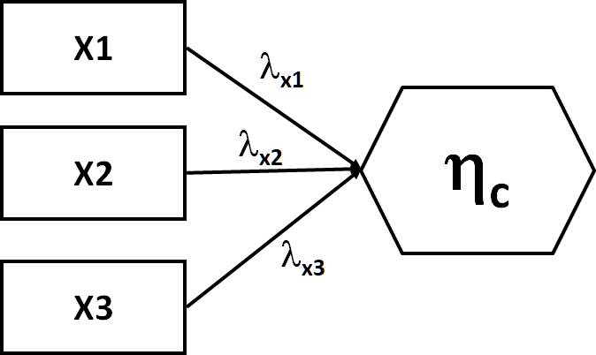
Here, the arrows are leading into, not out of, \(\eta\), indicating that the composite variable is made up of the influences of the three observed variables. Note: in this and other presentations, the composite is denoted by a hexagon, but can sometimes be an oval as it can technically be a form of a latent variable.
If the composite is entirely made up of the three influences, it can be said to have no error. An example might be the two levels of a treatment that lead into a single composite variable called ‘Treatment.’ In this case, there are no other levels of treatment because you, as the investigator, did not apply any. Thus the composite ‘treatment’ captures the full universe of treatment possibilities given the data.
In other cases, the property might arise from the collective influence of variables but is not without error. For example, the idea of soil condition arises from different aspects of the soil: its pH, moisture, grain size, and so on. However, one might measure only some of these, and thus there remain other factors (nutrient content, etc.) that might contribute to the notion of soil condition. In this case, the composite would have error and is therefore known as a latent composite.
The benefit of such an approach is that complicated constructs can be distilled into discrete blocks that are easier to present and discuss. For example, it is easier to talk about the effects of the experimental treatment on soil condition, rather than the effect of treatment 1 on soil moisture, the effect of treatment 1 on soil pH, the effect of treatment 1 on soil grain size, and so on.
In this way, the composite harkens back to the early meta-model, or broad conceptual relationships that inform the parameterization of the structural path model. In fact, in populating the meta-model, you may wish to consider those broad concepts as composites (or latents) when fitting the model, rather than modeling all relationships among all observed variables.
Selecting between latent and composite variables comes down to the concept in question, the presumed direction of causality, and the nature of the indicators.
For the soil example, consider: is it that there is a common difference among soils driving variation in pH, moisture, etc.? Or is it that pH, moisture, etc. are all independent properties that combine to inform soil condition? If the goal is measure plant growth in potting soils from different manufacturers, then manufacturer might be the common source of variation and a latent variable more appropriate. If the observer is visiting different sites and measuring conditions that describe the soil in each place, then perhaps a composite variable is warranted.
Another way of thinking about this is whether the indicators are interchangeable. In other words, does soil pH tell us the same information as soil moisture? If so, then they might be indicators of the same latent phenomenon. If not, and they contain unique information, then they likely combine to form a composite variable.
Finally, do the indicators co-vary? If they are under common control of a latent variable, then changing one should alter all the others. If they are relatively independent–for example, one could change grain size without changing nutrient content–then causation likely flows into a composite (rather than out of a latent) variable.
Now that we have defined a composite variable, let’s see how to make one.
8.2 Constructing a Composite Variable
Compared to latent variables, a composite variable is actually very easy to estimate: it is simply the sum of its indicators, hence the term composite.
The way in which the indicators are summed depends on whether they are expected to have the same weight (a fixed composite) or different weights (a statistical composite). The former might be something like species relative abundances. The latter is what we will focus on here because it has the most practical applications in ecology.
The weights for the composite are easily acquired as they are the values that maximize the explained variance in some response. We have done this before many times using maximum-likelihood fitting.
In fact, statistical composites can be boiled down to the coefficients from a multiple regression:
- The maximum-likelihood fitting function chooses parameter estimates for each predictor that maximize the likelihood of observing the response;
- Those parameter values serve as the loadings for the indicators of the composite variable;
- The data for each indicator are multiplied by their loading and summed to generate the factor scores for the composite variable, which is then used in the structural model.
Let’s demonstrate using some random data:
set.seed(8)

y <- rnorm(50)
x1 <- rnorm(50)
x2 <- x1 + runif(50)

# run multiple regression
model <- lm(y ~ x1 + x2)

# get loadings
beta_x1 <- summary(model)$coefficients[2, 1]

beta_x2 <-  summary(model)$coefficients[3, 1]

# compute factor scores
composite <- beta_x1 * x1 + beta_x2 * x2
These summed values can then used to predict the response:
summary(lm(y ~ composite))##
## Call:
## lm(formula = y ~ composite)
##
## Residuals:
## Min 1Q Median 3Q Max
## -2.88387 -0.70164 0.05644 0.54393 2.07769
##
## Coefficients:
## Estimate Std. Error t value Pr(>|t|)
## (Intercept) -0.3031 0.2424 -1.250 0.217
## composite 1.0000 0.8045 1.243 0.220
##
## Residual standard error: 1.014 on 48 degrees of freedom
## Multiple R-squared: 0.03118, Adjusted R-squared: 0.011
## F-statistic: 1.545 on 1 and 48 DF, p-value: 0.2199Note how the unstandardized coefficient is 1. This is because the composite is in units of the predicted values of the response. Thus, the coefficient is really only interpretable in standardized units.
Let’s alternately fit this composite model with lavaan and fix the loadings of \(x1\) and \(x2\) to the values from the multiple regression:
library(lavaan)

comp_formula1 <- '
composite <~ -0.498 * x1 + 0.579 * x2

y ~ composite
'

comp_model1 <- sem(comp_formula1, data.frame(y, x1, x2))

summary(comp_model1, standardize = T)
## lavaan 0.6-9 ended normally after 14 iterations
##
## Estimator ML
## Optimization method NLMINB
## Number of model parameters 2
##
## Number of observations 50
##
## Model Test User Model:
##
## Test statistic 0.000
## Degrees of freedom 1
## P-value (Chi-square) 0.999
##
## Parameter Estimates:
##
## Standard errors Standard
## Information Expected
## Information saturated (h1) model Structured
##
## Composites:
## Estimate Std.Err z-value P(>|z|) Std.lv Std.all
## composite <~
## x1 -0.498 -2.793 -3.163
## x2 0.579 3.248 3.642
##
## Regressions:
## Estimate Std.Err z-value P(>|z|) Std.lv Std.all
## y ~
## composite 1.000 0.788 1.269 0.205 0.178 0.177
##
## Variances:
## Estimate Std.Err z-value P(>|z|) Std.lv Std.all
## .y 0.987 0.197 5.000 0.000 0.987 0.969
## composite 0.000 0.000 0.000We see from the output that the estimated loadings for our two indicators are the same values we provided, and consequently the understandardized coefficient is 1. However, the standardized coefficient is 0.177 and it is this value that we would present (although its non-significant, given that these are fake data).
Let’s suppose we didn’t know the loadings from the multiple regression. We run into the same issue of identifiability as when constructing latent variables, so we must fix the first loading to 1. This will also define the scale of the composite. NOTE: lavaan does not do this automatically (as it does for latents), so we will have to implement it manually.
comp_formula2 <- '
composite <~ 1 * x1 + x2

y ~ composite
'

comp_model2 <- sem(comp_formula2, data.frame(y, x1, x2))
## Warning in lavaan::lavaan(model = comp_formula2, data = data.frame(y, x1, : lavaan WARNING:
## the optimizer warns that a solution has NOT been found!It seems that, because the true loading of \(x1\) on the composite is far from 1 (we know it is actually -0.498), we have received a non-convergence error!
One solution is to set the other loading to 1:
comp_formula3 <- '
composite <~ x1 + 1 * x2

y ~ composite
'

comp_model3 <- sem(comp_formula3, data.frame(y, x1, x2))

summary(comp_model3, standardize = T)
## lavaan 0.6-9 ended normally after 22 iterations
##
## Estimator ML
## Optimization method NLMINB
## Number of model parameters 3
##
## Number of observations 50
##
## Model Test User Model:
##
## Test statistic 0.000
## Degrees of freedom 0
##
## Parameter Estimates:
##
## Standard errors Standard
## Information Expected
## Information saturated (h1) model Structured
##
## Composites:
## Estimate Std.Err z-value P(>|z|) Std.lv Std.all
## composite <~
## x1 -0.860 0.230 -3.745 0.000 -2.792 -3.162
## x2 1.000 3.247 3.642
##
## Regressions:
## Estimate Std.Err z-value P(>|z|) Std.lv Std.all
## y ~
## composite 0.579 0.489 1.184 0.236 0.178 0.177
##
## Variances:
## Estimate Std.Err z-value P(>|z|) Std.lv Std.all
## .y 0.987 0.197 5.000 0.000 0.987 0.969
## composite 0.000 0.000 0.000Here the model converges because the true loading (0.579) is close enough to 1 for the maximum-likelihood fitting function to find it within a certain number of iterations.
Note that the unstandardized coefficient is no longer 1: this is because the scale of the composite has been set to that of the second indicator.
For reasons of model convergence, it is generally recommended that one compute the loadings by hand and fix them in the model. This has an added benefit we will get to in a later section. But first let’s explore a real-world example.
8.3 Grace & Keeley Revisited: A Worked Example
Recall from the chapters on global and local estimation that Grace & Keeley (2006) were interested in the factors that mediated recovery of shrublands post-fire disturbance. In those chapters, we fit different sub-models of their larger model, and we’ll fit a different sub-model yet again in this chapter for simplicity.
In their model, they used plant cover to predict plant species richness. Let’s assume for a moment that the relationship between cover and richness may be non-linear: its not until a certain amount of cover that rarer species begin to appear, for example. In this case, we might suppose there are both linear \(cover\) and non-linear \(cover^2\) components to the model. Composite variables are a nice way to summarize both the linear and non-linear effects.
Let’s fit the following composite variable:
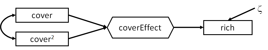
Here we have a composite that summarizes the unsquared and squared values of cover, which then goes on to predict richness.
Let’s adopt the two-step approach and first fit a linear model.
library(piecewiseSEM)

data(keeley)

cover_model <- lm(rich ~ cover + I(cover^2), keeley)

summary(cover_model)
##
## Call:
## lm(formula = rich ~ cover + I(cover^2), data = keeley)
##
## Residuals:
## Min 1Q Median 3Q Max
## -29.161 -11.958 -0.595 10.094 32.956
##
## Coefficients:
## Estimate Std. Error t value Pr(>|t|)
## (Intercept) 25.641 6.574 3.900 0.000189 ***
## cover 57.999 18.931 3.064 0.002910 **
## I(cover^2) -28.577 12.385 -2.307 0.023403 *
## ---
## Signif. codes: 0 '***' 0.001 '**' 0.01 '*' 0.05 '.' 0.1 ' ' 1
##
## Residual standard error: 14 on 87 degrees of freedom
## Multiple R-squared: 0.1598, Adjusted R-squared: 0.1404
## F-statistic: 8.271 on 2 and 87 DF, p-value: 0.0005147It seems both the unsquared and squared values of cover significantly predict richness, so we are justified in including both as indicators to our composite variable. Now we extract the coefficients, use them to generate the factor scores, and finally use those scores to predict richness.
beta_cover <- summary(cover_model)$coefficients[2, 1]

beta_cover2 <- summary(cover_model)$coefficients[3, 1]

composite <- beta_cover * keeley$cover + beta_cover2 * (keeley$cover)^2

summary(lm(rich ~ composite, data = data.frame(keeley, composite)))
##
## Call:
## lm(formula = rich ~ composite, data = data.frame(keeley, composite))
##
## Residuals:
## Min 1Q Median 3Q Max
## -29.161 -11.958 -0.595 10.094 32.956
##
## Coefficients:
## Estimate Std. Error t value Pr(>|t|)
## (Intercept) 25.6406 5.9516 4.308 4.27e-05 ***
## composite 1.0000 0.2445 4.090 9.51e-05 ***
## ---
## Signif. codes: 0 '***' 0.001 '**' 0.01 '*' 0.05 '.' 0.1 ' ' 1
##
## Residual standard error: 13.93 on 88 degrees of freedom
## Multiple R-squared: 0.1598, Adjusted R-squared: 0.1502
## F-statistic: 16.73 on 1 and 88 DF, p-value: 9.507e-05As would be expected from the multiple regression, the composite term significantly predicts richness (P < 0.001). Let’s use the coefs function from piecewiseSEM to obtain the standardized coefficient:
coefs(lm(rich ~ composite, data = data.frame(keeley, composite)))## Response Predictor Estimate Std.Error DF Crit.Value P.Value Std.Estimate
## 1 rich composite 1 0.2445 88 4.0904 1e-04 0.3997 ***So a 1 standard deviation change in the total cover effect would result in a 0.40 standard deviation change in plant richness.
We can alternately fit the model with lavaan using the same coefficients from the multiple regression:
# create a new non-linear variable for cover^2
keeley$coversq <- keeley$cover^2

keeley_formula1 <- '
composite <~ 58 * cover + -28.578 * coversq

rich ~ composite
'

keeley_model1 <- sem(keeley_formula1, keeley, fixed.x = F)

summary(keeley_model1, standardize = T)
## lavaan 0.6-9 ended normally after 20 iterations
##
## Estimator ML
## Optimization method NLMINB
## Number of model parameters 5
##
## Number of observations 90
##
## Model Test User Model:
##
## Test statistic 0.000
## Degrees of freedom 1
## P-value (Chi-square) 1.000
##
## Parameter Estimates:
##
## Standard errors Standard
## Information Expected
## Information saturated (h1) model Structured
##
## Composites:
## Estimate Std.Err z-value P(>|z|) Std.lv Std.all
## composite <~
## cover 58.000 9.660 3.048
## coversq -28.578 -4.760 -2.295
##
## Regressions:
## Estimate Std.Err z-value P(>|z|) Std.lv Std.all
## rich ~
## composite 1.000 0.242 4.137 0.000 6.004 0.400
##
## Covariances:
## Estimate Std.Err z-value P(>|z|) Std.lv Std.all
## cover ~~
## coversq 0.147 0.022 6.602 0.000 0.147 0.969
##
## Variances:
## Estimate Std.Err z-value P(>|z|) Std.lv Std.all
## .rich 189.597 28.263 6.708 0.000 189.597 0.840
## composite 0.000 0.000 0.000
## cover 0.100 0.015 6.708 0.000 0.100 1.000
## coversq 0.233 0.035 6.708 0.000 0.233 1.000Which leads us to the same standardized coefficient (0.40) as through the manual calculation.
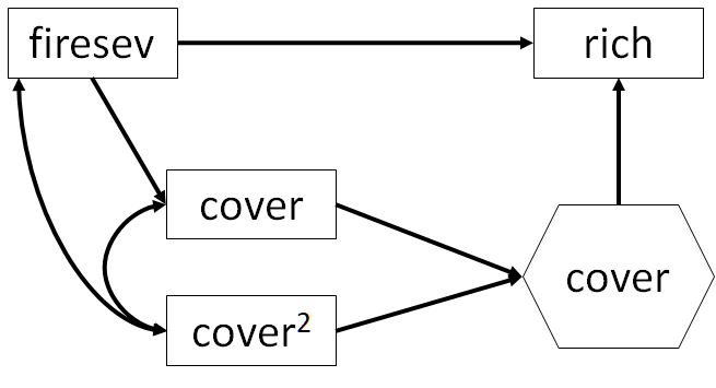
Finally, let’s incorporate the effect of fire severity on cover and richness. Now the composite is endogenous because it is affected by fire severity, and goes on to predict richness.
First, we must fit the model without the composite to get the loadings of \(cover\) and \(cover^2\).
keeley_formula2 <- '
composite <~ 58 * cover + -28.578 * coversq

rich ~ composite + firesev

cover ~ firesev

cover ~~ coversq

firesev ~~ coversq
'

keeley_model2 <- sem(keeley_formula2, keeley)

summary(keeley_model2, standardize = T, rsq = T)
## lavaan 0.6-9 ended normally after 53 iterations
##
## Estimator ML
## Optimization method NLMINB
## Number of model parameters 9
##
## Number of observations 90
##
## Model Test User Model:
##
## Test statistic 0.065
## Degrees of freedom 1
## P-value (Chi-square) 0.799
##
## Parameter Estimates:
##
## Standard errors Standard
## Information Expected
## Information saturated (h1) model Structured
##
## Composites:
## Estimate Std.Err z-value P(>|z|) Std.lv Std.all
## composite <~
## cover 58.000 9.660 3.048
## coversq -28.578 -4.760 -2.295
##
## Regressions:
## Estimate Std.Err z-value P(>|z|) Std.lv Std.all
## rich ~
## composite 0.731 0.265 2.757 0.006 4.391 0.292
## firesev -2.132 0.969 -2.200 0.028 -2.132 -0.233
## cover ~
## firesev -0.084 0.018 -4.611 0.000 -0.084 -0.437
##
## Covariances:
## Estimate Std.Err z-value P(>|z|) Std.lv Std.all
## .cover ~~
## coversq 0.122 0.019 6.588 0.000 0.122 0.893
## coversq ~~
## firesev -0.301 0.089 -3.369 0.001 -0.301 -0.380
##
## Variances:
## Estimate Std.Err z-value P(>|z|) Std.lv Std.all
## .rich 179.922 26.821 6.708 0.000 179.922 0.797
## .cover 0.081 0.012 6.708 0.000 0.081 0.809
## coversq 0.233 0.035 6.708 0.000 0.233 1.000
## firesev 2.700 0.402 6.708 0.000 2.700 1.000
## composite 0.000 0.000 0.000
##
## R-Square:
## Estimate
## rich 0.203
## cover 0.191Note that the squared and unsquared terms for \(cover\) have correlated errors, because they are both driven by the underlying values of cover. Also, because the squared term is not a ‘true’ variable in the model but a convenience for us to explore this non-linearity, we must treat \(cover\) and \(cover^2\) as exogenous even though they are part of an endogenous composite. lavaan automatically models correlations among exogenous variables, but will not do so for the composite indicators unless told explicitly. In this case, then, we must manually control for the correlation between \(cover^2\) and \(cover\) and \(firesev\).
Here, we find a good-fitting model (P = 0.80). Moreover, we obtain the standardized coefficient for the effect of fire severity on cover \(\gamma = -0.437\) and of the composite on richness \(\beta = 0.292\) controlling for fire severity, which is the total non-linear effect of cover.
To otain the indirect effect then, we multiply these paths plus the standardized loading \(cover\) on the composite: \(-0.437 * 3.048 * 0.292 = -0.389\).
8.4 Composites in piecewiseSEM
For the moment, composites are not directly implemented in piecewiseSEM with special syntax like in lavaan, but we hope to introduce that functionality soon. In the interim, they are easy to compute them by hand, as we have shown above, extract the predicted scores, and use them as any other predictor.
Let’s examine this with the Keeley model as above:
keeley$composite <- composite

keeley_psem <- psem(
  lm(cover ~ firesev, keeley),
  lm(rich ~ composite + firesev, keeley)
)

summary(keeley_psem, .progressBar = FALSE)
##
## Structural Equation Model of keeley_psem
##
## Call:
## cover ~ firesev
## rich ~ composite + firesev
##
## AIC
## 765.393
##
## ---
## Tests of directed separation:
##
## Independ.Claim Test.Type DF Crit.Value P.Value
## cover ~ composite + ... coef 87 11.6011 0.0000 ***
## rich ~ cover + ... coef 86 -0.2497 0.8034
##
## --
## Global goodness-of-fit:
##
## Chi-Squared = 84.206 with P-value = 0 and on 2 degrees of freedom
## Fisher's C = 86.213 with P-value = 0 and on 4 degrees of freedom
##
## ---
## Coefficients:
##
## Response Predictor Estimate Std.Error DF Crit.Value P.Value Std.Estimate
## cover firesev -0.0839 0.0184 88 -4.5594 0.0000 -0.4371 ***
## rich composite 0.7314 0.2698 87 2.7108 0.0081 0.2923 **
## rich firesev -2.1323 0.9859 87 -2.1629 0.0333 -0.2332 *
##
## Signif. codes: 0 '***' 0.001 '**' 0.01 '*' 0.05
##
## ---
## Individual R-squared:
##
## Response method R.squared
## cover none 0.19
## rich none 0.20Note that we get the same standardized coefficients as in lavaan! There is, however, deviation in the goodness-of-fit that are accounted for by differences in how the composite is constructed and the correlated errors among the indicator and \(firesev\) which are not possible to model in piecewiseSEM yet.
8.5 References
Grace, J. B., & Keeley, J. E. (2006). A structural equation model analysis of postfire plant diversity in California shrublands. Ecological Applications, 16(2), 503-514.